
# def 添加层 如何构造神经网络 并展示拟合过程
import tensorflow as tf
import numpy as np
import matplotlib.pyplot as plt  # 若没有 pip install matplotlib


# 定义一个神经层
def add_layer(inputs, in_size, out_size, activation_function=None):
    #add one more layer and return the output of the layer
    Weights = tf.Variable(tf.random_normal([in_size, out_size])) #in_size:上一层的节点数  out_size:当前的节点数
    biases = tf.Variable(tf.zeros([1, out_size]) + 0.1)
    Wx_plus_b = tf.matmul(inputs, Weights) + biases
    if activation_function is None:
        outputs = Wx_plus_b
    else:
        outputs = activation_function(Wx_plus_b)
    return outputs

# x_data值为-1到1之间,有300个单位(例子),即为1*300的行向量,
# 通过[:, np.newaxis],再加一个维度newaxis,即300*1的列向量
x_data = np.linspace(-1, 1, 300)[:, np.newaxis]
noise = np.random.normal(0, 0.05, x_data.shape)  # 均值为0.方差为0.05,格式和x_data一样
y_data = np.square(x_data) - 0.5 + noise

#1是指的数据的尺寸,None指的batch size的大小,所以可以是任何数,无论给多少个例子都行
xs = tf.placeholder(tf.float32, [None, 1])
ys = tf.placeholder(tf.float32, [None, 1])

# 设置输入层,隐藏层,输出层
# 输入层
l1 = add_layer(xs, 1, 10, activation_function=tf.nn.relu)
# 输出层
prediction = add_layer(l1, 10, 1, activation_function=None)

loss = tf.reduce_mean(
    # 对每个例子进行求和并取平均值
    # reduction_indices参数,表示函数的处理维度,
    # reduction_indices=[1]指按行求和reduction_indices=[0]指按列求和
    # 如果代码中并没有reduction_indices这个参数,该参数取默认值None,将把input_tensor降到0维,也就是一个数,即对所有数求和
    tf.reduce_sum(tf.square(ys - prediction), reduction_indices=[1]))
train_step = tf.train.GradientDescentOptimizer(0.1).minimize(loss)  # 以0.1的学习效率对误差进行更正和提升

#两种初始化的方式
#init = tf.initialize_all_variables()
init = tf.global_variables_initializer()
sess = tf.Session()
sess.run(init)

fig = plt.figure()
# 将figure设置的画布大小分成几个部分,
# plt.subplot(2,2,1)参数‘221’表示2(row)x2(colu),即将画布分成2x2,两行两列的4块区域,1表示选择图形输出的区域在第一块,
# 图形输出区域参数必须在“行x列”范围内,
# 此处必须在1和2之间选择——如果参数设置为subplot(1,1,1),则表示画布整个输出,不分割成小块区域,图形直接输出在整块画布上
ax = fig.add_subplot(1, 1, 1)
#设置画布的输入的数据为x_data y_data
ax.scatter(x_data, y_data)
#在使用matplotlib的过程中,常常会需要画很多图,但是好像并不能同时展示许多图。 这是因为python可视化库matplotlib的显示模式默认为阻塞(block)模式。
# 什么是阻塞模式那?我的理解就是在plt.show()之后,程序会暂停到那儿,并不会继续执行下去。如果需要继续执行程序,就要关闭图片。
# 那如何展示动态图或多个窗口呢?这就要使用plt.ion()这个函数,使matplotlib的显示模式转换为交互(interactive)模式。即使在脚本中遇到plt.show(),代码还是会继续执行。
plt.ion()
plt.show()

for i in range(1000):
    sess.run(train_step, feed_dict={xs: x_data, ys: y_data})
    if i % 50 == 0:
        # to see the step improment 显示实际点的数据
        print(sess.run(loss,feed_dict = {xs:x_data,ys:y_data}))
        try:
            # 每次划线前抹除上一条线,抹除lines的第一条线,由于lines只有一条线,则为lines[0],第一次没有线
            ax.lines.remove(lines[0])
        except Exception:
            pass
        # 显示预测数据
        prediction_value = sess.run(prediction, feed_dict={xs: x_data})

        # 存储 prediction_value 的值
        lines = ax.plot(x_data, prediction_value, 'r-', lw=5)  # 用红色的线画,且宽度为5

        # 停止0.1秒后再画下一条线
        plt.pause(0.1)
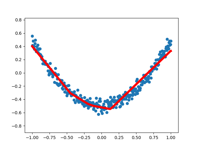
实验结果图展示:
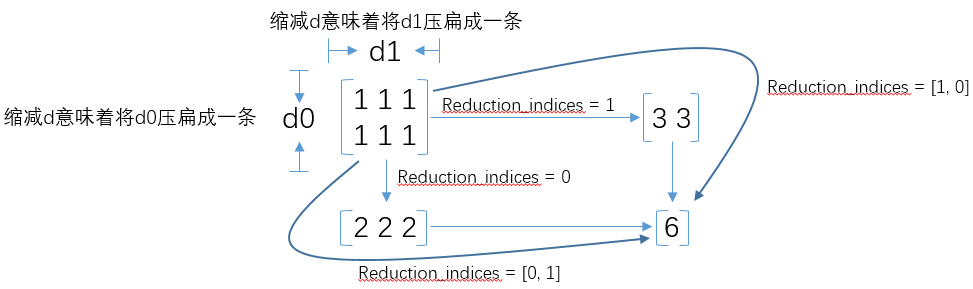
附:参考https://www.cnblogs.com/likethanlove/p/6547405.html 通过图可以加深对tensorflow reduction_indices的理解:

 浙公网安备 33010602011771号