GRU&实例股价预测

GRU 由 Cho 等人于 2014 年提出，优化 LSTM 结构。

Kyunghyun Cho,Bart vanMerrienboer,Caglar Gulcehre,Dzmitry Bahdanau,Fethi Bougares,HolgerSchwenk,Yoshua Bengio.Learning Phrase Representations using RNNEncoder–Decoder for Statistical Machine Translation.Computer ence,2014

1.原理

门控循环单元(Gated Recurrent Unit， GRU)是 LSTM 的一种变体，将 LSTM 中遗忘门与输入门合二为一为更新门，模型比 LSTM 模型更简单。

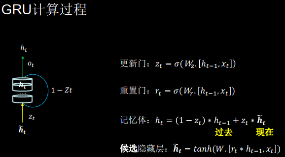
　　　　　　　　　　　　　　　　图 2.3.1 GRU 计算过程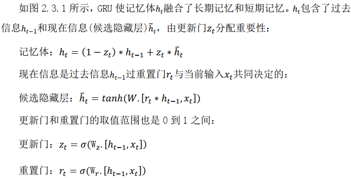

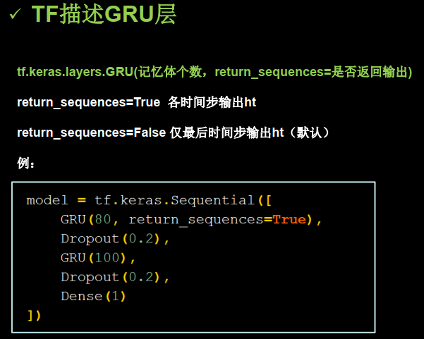
2.TF描述GRU层

3.代码实现

改变的地方

100

101

102

103

104

105

106

107

108

109

110

111

112

113

114

115

116

117

118

119

120

121

122

123

124

125

126

127

128

129

130

131

132

133

134

135

136

137

138

139

140

141

142

143

144

145

146

147

148

149

150

151

152

153

154

155

156

157

158

159

160

161

162

163

164

165

166

#! /usr/bin/env python
# -*- coding:utf-8 -*-
# __author__ = "yanjungan"
 
 
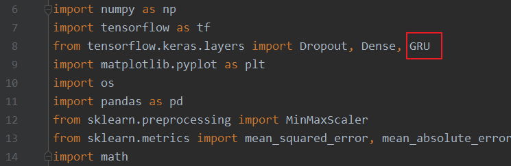
import numpy as np
import tensorflow as tf
from tensorflow.keras.layers import Dropout, Dense, GRU
import matplotlib.pyplot as plt
import os
import pandas as pd
from sklearn.preprocessing import MinMaxScaler
from sklearn.metrics import mean_squared_error, mean_absolute_error
import math
 
# 读取股票文件
maotai = pd.read_csv('./datasets/SH600519.csv')
 
# 前(2426-300=2126)天的开盘价作为训练集，表格从0开始计数，2:3是提取[2:3]列，前闭后开，故提取出c列开盘价
training_set = maotai.iloc[0:2426 - 300, 2:3].values
# 后300天数据
test_set = maotai.iloc[2426 - 300:, 2:3].values
 
# 归一化
# 定义归一化，归一化到(0，1)之间
sc = MinMaxScaler(feature_range=(0, 1))
# 求得训练集的最大值，最小值这些训练集固有的属性，并在训练集上进行归一化
training_set_scaled = sc.fit_transform(training_set)
# 利用训练集的属性对测试集进行归一化
test_set = sc.transform(test_set)
 
x_train = []
y_train = []
 
x_test = []
y_test = []
 
# 训练集：csv表格中前2426-300=2126天数据
# 利用for循环，遍历整个训练集，提取训练集中连续60天的开盘价作为输入特征x_train，
# 第61天的数据作为标签，for循环共构建2426-300-60=2066组数据。
for i in range(60, len(training_set_scaled)):
    x_train.append(training_set_scaled[i - 60:i, 0])
    y_train.append(training_set_scaled[i, 0])
 
# 打乱训练集数据
np.random.seed(7)
np.random.shuffle(x_train)
np.random.seed(7)
np.random.shuffle(y_train)
tf.random.set_seed(7)
 
# 将训练集由list变成array格式
x_train, y_train = np.array(x_train), np.array(y_train)
 
# 使x_train符合RNN输入要求：[送入样本数， 循环核时间展开步数， 每个时间步输入特征个数]。
# 此处整个数据集送入，送入样本数为x_train.shape[0]即2066组数据；输入60个开盘价，预测出第61天的开盘价，循环核时间展开步数为60;
# 每个时间步送入的特征是某一天的开盘价，只有1个数据，故每个时间步输入特征个数为1
x_train = np.reshape(x_train, (x_train.shape[0], 60, 1))
 
# 测试集：csv表格中后300天数据
# 利用for循环，遍历整个测试集，提取测试集中连续60天的开盘价作为输入特征x_train，第61天的数据作为标签，for循环共构建300-60=240组数据。
for i in range(60, len(test_set)):
    x_test.append(test_set[i - 60:i, 0])
    y_test.append(test_set[i, 0])
 
# 将测试集由list变成array格式
x_test, y_test = np.array(x_test), np.array(y_test)
 
# 测试集变array并reshape为符合RNN输入要求：[送入样本数， 循环核时间展开步数， 每个时间步输入特征个数]
x_test = np.reshape(x_test, [x_test.shape[0], 60, 1])
 
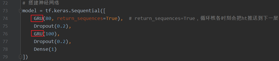
# 搭建神经网络
model = tf.keras.Sequential([
    GRU(80, return_sequences=True),  # return_sequences=True，循环核各时刻会把ht推送到下一层
    Dropout(0.2),
    GRU(100),
    Dropout(0.2),
    Dense(1)
])
 
# 配置训练方法
model.compile(
    optimizer=tf.keras.optimizers.Adam(0.001),
    loss='mean_squared_error'  # 损失函数用均方误差
)
# 该应用只观测loss数值，不观测准确率，所以删去metrics选项，一会在每个epoch迭代显示时只显示loss值
 
# 保存模型
checkpoint_path_save = './checkpoint/gru_stock.ckpt'
 
# 如果模型存在，就加载模型
if os.path.exists(checkpoint_path_save + '.index'):
    print('--------------------load the model----------------------')
    # 加载模型
    model.load_weights(checkpoint_path_save)
 
# 保存模型，借助tensorflow给出的回调函数，直接保存参数和网络
'''
 注： monitor 配合 save_best_only 可以保存最优模型，
 包括：训练损失最小模型、测试损失最小模型、训练准确率最高模型、测试准确率最高模型等。
'''
cp_callback = tf.keras.callbacks.ModelCheckpoint(
    filepath=checkpoint_path_save,
    save_weights_only=True,
    save_best_only=True,
    monitor='val_loss'
)
 
# 模型训练
history = model.fit(x_train, y_train,
                    batch_size=64, epochs=50, validation_data=(x_test, y_test),
                    validation_freq=1, callbacks=[cp_callback])
 
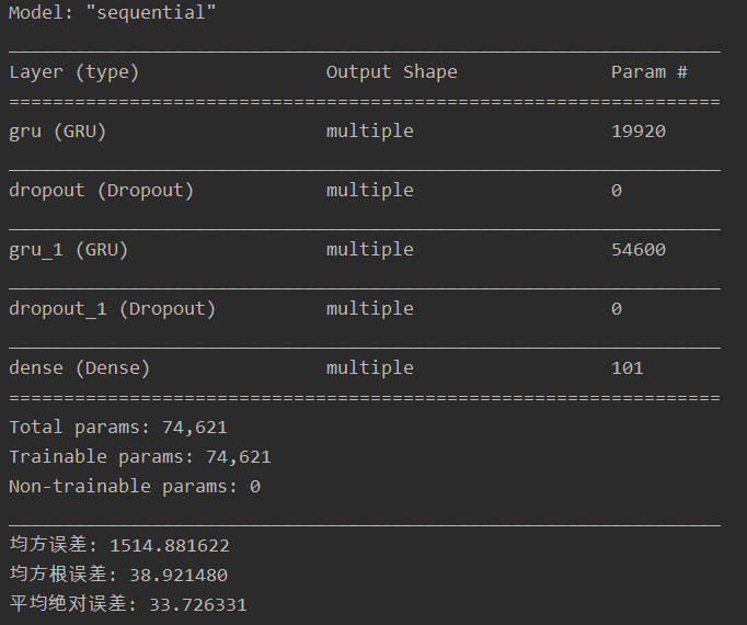
# 统计网络结构参数
model.summary()
 
# 参数提取，写至weights_stock.txt文件中
file = open('./gru_weights_stock.txt', 'w')
for v in model.trainable_variables:
    file.write(str(v.name) + '\n')
    file.write(str(v.shape) + '\n')
    file.write(str(v.numpy()) + '\n')
file.close()
 
# 获取loss
loss = history.history['loss']
val_loss = history.history['val_loss']
 
# 绘制loss
plt.plot(loss, label='Training Loss')
plt.plot(val_loss, label='Validation Loss')
plt.title('Training and Validation Loss')
plt.legend()
plt.show()
 
######################## predict ###################################
 
# 测试集输入到模型中进行预测
predicted_stock_price = model.predict(x_test)
 
# 对预测数据还原---从(0, 1)反归一化到原始范围
predicted_stock_price = sc.inverse_transform(predicted_stock_price)
 
# 对真实数据还原---从(0, 1)反归一化到原始范围
real_stock_price = sc.inverse_transform(test_set[60:])
 
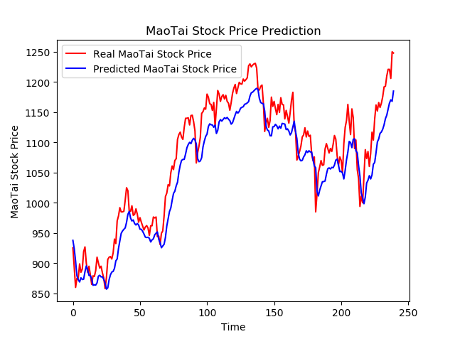
# 画出真实数据和预测数据的对比曲线
plt.plot(real_stock_price, color='red', label='Real MaoTai Stock Price')
plt.plot(predicted_stock_price, color='blue', label='Predicted MaoTai Stock Price')
plt.title('MaoTai Stock Price Prediction')
plt.xlabel('Time')
plt.ylabel('MaoTai Stock Price')
plt.legend()
plt.show()
 
###################### evluate ######################
# calculate MSE 均方误差 ---> E[(预测值-真实值)^2] (预测值减真实值求平方后求均值)
mse = mean_squared_error(predicted_stock_price, real_stock_price)
# calculate RMSE 均方根误差--->sqrt[MSE]    (对均方误差开方)
rmse = math.sqrt(mean_squared_error(predicted_stock_price, real_stock_price))
# calculate MAE 平均绝对误差----->E[|预测值-真实值|](预测值减真实值求绝对值后求均值）
mae = mean_absolute_error(predicted_stock_price, real_stock_price)
 
print('均方误差: %.6f' % mse)
print('均方根误差: %.6f' % rmse)
print('平均绝对误差: %.6f' % mae)