
Series和DataFrame的简单数学运算:
import numpy as np
import pandas as pd
Series的运算:
n = np.nan
n = 1
m+n      #nan加任何数都是nan
---------------
nan
s1 = pd.Series([1,2,3],index=['a','b','c'])
s2 = pd.Series([4,5,6,7],index=["B","C","D","E"])
print(s1)
print(s2)
---------------------------------------------
A    1
B    2
C    3

B    4
C    5
D    6
E    7
如果index对应就相加,没有对应的index则变成NaN
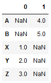
s3 = s1+s2
print(s3)
-------------------
A    NaN
B    6.0
C    8.0
D    NaN
E    NaN
DataFrame的运算:
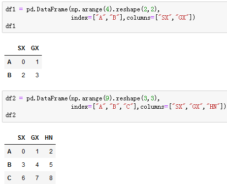
df3 = df1 + df2
print(df3)
---------------------
      GX      HN      SX
_________________________
A     2.0     NaN     0.0
B     7.0     NaN     5.0
C     NaN     NaN     NaN
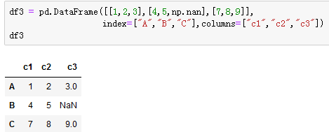
s1 = df3.sum()  #计算每个columns的和
print(s1)
------------------------
c1    12.0
c2    15.0
c3    12.0
s2 = df3.sum(axis=1) #计算行的总和,默认是0
print(s2)
------------------------------------
A     6.0
B     9.0
C    24.0
s1 = df3.sum(axis=0,skipna=False)  #skipna是否跳过NaN计算
print(s1)
------------------------------------
c1    12.0
c2    15.0
c3     NaN
Series和Dataframe的排序:
Series的排序:
s1 = pd.Series(np.random.randn(10))
print(s1)
------------------------------
0   -0.228264
1    0.087456
2   -0.717422
3    0.126064
4   -0.190748
5   -0.600853
6    0.201084
7    0.152117
8   -0.349236
9   -0.120914
s2 = s1.short_values(ascending=False) #按values排序,默认升序True,False是降序
print(s2)
-------------------------------
6    0.201084
7    0.152117
3    0.126064
1    0.087456
9   -0.120914
4   -0.190748
0   -0.228264
8   -0.349236
5   -0.600853
2   -0.717422
s1.sort_values(ascending=False,inplace=True) #inplace是否对原值修改,默认False不对原值修改
print(s1)
--------------------------------
6    0.201084
7    0.152117
3    0.126064
1    0.087456
9   -0.120914
4   -0.190748
0   -0.228264
8   -0.349236
5   -0.600853
2   -0.717422
s1.sort_index()   #按index排序
------------------------
0   -0.228264
1    0.087456
2   -0.717422
3    0.126064
4   -0.190748
5   -0.600853
6    0.201084
7    0.152117
8   -0.349236
9   -0.120914
DataFrame的排序:
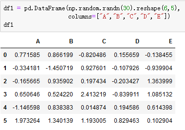
df2 = df1['A'].sort_values()     #取出A列的值,按values升序排列
print(df2)
---------------------------------
4   -1.146598
1   -0.334181
2   -0.165665
3    0.650646
0    0.771585
5    1.973264
df2.sort_index()
-------------------
0    0.771585
1   -0.334181
2   -0.165665
3    0.650646
4   -1.146598
5    1.973264
DataFrame融合:
import pandas as pd
import numpy as np
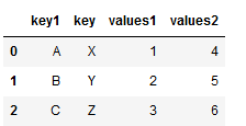
将两个DataFrame融合必须要有一个公共的列,否则会报错,且公共列中至少有一个值相等,不然融合出现的是空列表
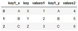
df1 = pd.DataFrame({"key1":["A","B","C"],"key":["X","Y","Z"],"values1":[1,2,3]})
df2 = pd.DataFrame({"key1":["A","B","C"],"key":["X","Y","Z"],"values2":[4,5,6]})
print(df1)
print(df2)
pd.merge(df1,df2)  #融合
------------------------------------
  key1 key  values1
0    A   X        1
1    B   Y        2                   <-----df1
2    C   Z        3

  key1 key  values2
0    A   X        4
1    B   Y        5                   <-----df2
2    C   Z        6
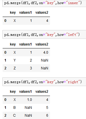
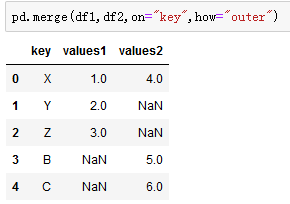
pd.merge(df1,df2,on='key') #指定一个融合的公共列
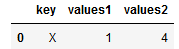
df1 = pd.DataFrame({"key":["X","Y","Z"],"values1":[1,2,3]})
df2 = pd.DataFrame({"key":["X","B","C"],"values2":[4,5,6]})
print(df1)
print(df2)
pd.merge(df1,df2)
----------------------------------
  key  values1
0   X        1
1   Y        2                <-----df1
2   Z        3

  key  values2
0   X        4
1   B        5                <-----df2
2   C        6
连接和组合:
numpy的数组连接
import numpy as np
import pandas as pd
arr1 = np.arange(9).reshape(3,3)
arr2 = arr1
print(np.concatenate([arr1,arr2]))  #默认 axis=0纵向连接
print(np.concatenate([arr1,arr2],axis=1))  #横向连接
--------------------------------------------------------------
[[ 0  1  2]
 [ 3  4  5]
 [ 6  7  8]
 [ 9 10 11]
 [ 0  1  2]
 [ 3  4  5]
 [ 6  7  8]]

[[0, 1, 2, 0, 1, 2],
 [3, 4, 5, 3, 4, 5],
 [6, 7, 8, 6, 7, 8]]
横向连接必须行数相同,纵向连接必须列数相同,不然会报错
Series的连接Contatenate
s1 = pd.Series([1,2,3],index=['X','Y','Z'])
s2 = pd.Series([4,5],index=['A','B'])
print(pd.concat([s1,s2]))
print(pd.concat([s2,s1]))
--------------------------------------
X    1
Y    2
Z    3                <-----s1,s2
A    4
B    5

A    4
B    5
X    1                <-----s2,s1
Y    2
Z    3
pd.concat([s1,s2],axis=1,sort=True)
DataFrame的连接Contatenate
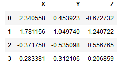
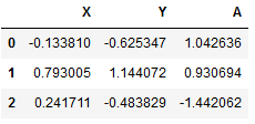
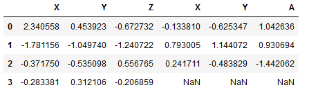
df1 = pd.DataFrame(np.random.randn(4,3),columns=["X","Y","Z"])
df2 = pd.DataFrame(np.random.randn(3,3),columns=["X","Y","A"])
print(df1)
print(df2)
---------------------------------------------
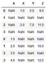
print(pd.concat([df1,df2],sort=True))
print(pd.concat([df1,df2],axis=1))
Series的Combine组合
s1 = pd.Series([2,np.nan,4,np.nan],index=["A","B","C","D"])
s2 = pd.Series([1,2,3,4],index=["A","B","C","D"])
print(s1)
print(s2)
-----------------------------
A    2.0
B    NaN     <-----s1
C    4.0
D    NaN

A    1
B    2       <-----s2
C    3
D    4
s1.combine_first(s2)   #将s2和s1组合,如果s1有nan值,则用s2同位置的值填充
------------------------------
A    2.0
B    2.0
C    4.0
D    4.0
s2.combine_first(s1)
-------------------------
A    1.0
B    2.0
C    3.0
D    4.0
DataFrame的组合Combine
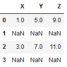
df1 = pd.DataFrame({"X":[1,np.nan,3,np.nan],
"Y":[5,np.nan,7,np.nan],
"Z":[9,np.nan,11,np.nan]})
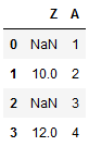
df2 = pd.DataFrame({"Z":[np.nan,10,np.nan,12],
"A":[1,2,3,4]})
print(df1)
print(df2)
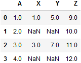
df1.combine_first(df2) #在df1数据前面组合df2
通过apply进行数据预处理:
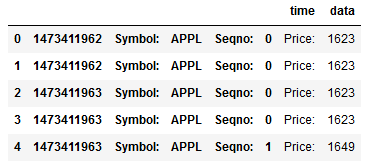
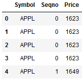
#复制以下数据
         time                                data
0  1473411962   Symbol: APPL Seqno: 0 Price: 1623
1  1473411962   Symbol: APPL Seqno: 0 Price: 1623
2  1473411963   Symbol: APPL Seqno: 0 Price: 1623
3  1473411963   Symbol: APPL Seqno: 0 Price: 1623
4  1473411963   Symbol: APPL Seqno: 1 Price: 1649
import numpy as np
import pandas as pd
df = pd.read_clipboard()   #读取复制的数据
print(df)


df.to_csv("apply_demo.csv")
df = pd.read_csv("apply_demo.csv")
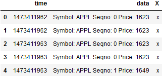
s1 = pd.Series(['x']*5)
df['x'] = s1.values    #给df添加一列,内容是s1的values
df
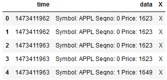
df['X'] = df['X'].apply(str.upper)   #将df的X列的值当做参数,全部upper
df
l1 = df["data"][0]
print(l1)
l1 = df["data"][0].split(" ")
print(l1)
--------------------------
'Symbol: APPL Seqno: 0 Price: 1623'

['Symbol:', 'APPL', 'Seqno:', '0', 'Price:', '1623']
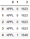
def foo(line):
    items = line.split(' ')
    return pd.Series([items[1],items[3],items[5]])
df_tmp = df['data'].apply(foo) #将每行的data列当做foo参数
df_tmp
df_tmp.rename(columns={0:'Symbol',1:'Seqno',2:'Price'})
#重新定义每个columns的名字
df_tmp
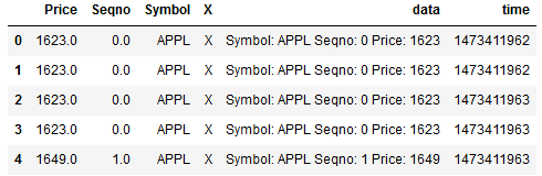
df_new = df.combine_first(df_tmp)  #在df前面组合df_tmp
df_new
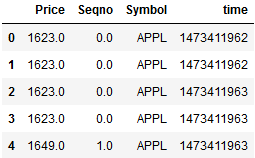
del df_new['data']
del df_new['X']
def_new
通过去重进行数据清理
import numpy as np
import pandas as pd
这里使用上面的df数据
df['Seqno'].unique()  #通过unique将Seqno列的重复值去除返回剩下的值
-------------------------
[0.,1.]
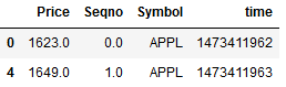
df["Seqno"].duplicated()   #查看是否为重复值
df.drop_duplicates(['Seqno'])  #去除Seqno有重复值的行
时间序列的操作基础
import numpy as np
import pandas as pd
from datetime import datetime
date_list = [datetime(2017,3,1),datetime(2018,3,1),datetime(2018,6,20),
            datetime(2018,7,2),datetime(2018,10,1),datetime(2018,10,9)]
s1 = pd.Series(np.random.randn(6),index=date_list)
print(s1)
---------------------------------------
2017-03-01    0.664216
2018-03-01    0.259339
2018-06-20    0.710367
2018-07-02    0.920019
2018-10-01   -0.297789
2018-10-09    1.337095
print(s1['2018-10-09'])
print(s1['2018-10'])
print(s1['2018'])
-----------------------------
1.3370947151802048

2018-10-01   -0.297789
2018-10-09    1.337095

2018-03-01    0.259339
2018-06-20    0.710367
2018-07-02    0.920019
2018-10-01   -0.297789
2018-10-09    1.337095
#批量生产日期数据
data_list_new = pd.date_range(start='2018-01-01',end = '2018-01-31')
print(date_list_new)
s2 = pd.Series(np.random.rand(),index=date_list_new)
print(s2)
------------------------------------------
['2018-01-01', '2018-01-02', '2018-01-03', '2018-01-04',
'2018-01-05', '2018-01-06', '2018-01-07', '2018-01-08',
'2018-01-09', '2018-01-10', '2018-01-11', '2018-01-12',
'2018-01-13', '2018-01-14', '2018-01-15', '2018-01-16', '2018-01-17', '2018-01-18', '2018-01-19', '2018-01-20',
'2018-01-21', '2018-01-22', '2018-01-23', '2018-01-24',
'2018-01-25', '2018-01-26', '2018-01-27', '2018-01-28',
'2018-01-29', '2018-01-30', '2018-01-31']

2018-01-01    0.810988
2018-01-02    0.810988
2018-01-03    0.810988
2018-01-04    0.810988
2018-01-05    0.810988
2018-01-06    0.810988
2018-01-07    0.810988
2018-01-08    0.810988
2018-01-09    0.810988
2018-01-10    0.810988
2018-01-11    0.810988
2018-01-12    0.810988
2018-01-13    0.810988
2018-01-14    0.810988
2018-01-15    0.810988
2018-01-16    0.810988
2018-01-17    0.810988
2018-01-18    0.810988
2018-01-19    0.810988
2018-01-20    0.810988
2018-01-21    0.810988
2018-01-22    0.810988
2018-01-23    0.810988
2018-01-24    0.810988
2018-01-25    0.810988
2018-01-26    0.810988
2018-01-27    0.810988
2018-01-28    0.810988
2018-01-29    0.810988
2018-01-30    0.810988
2018-01-31    0.810988
t_range = pd.date_range("2018-01-01","2018-12-31")
print(t_range)
----------------------------------
['2018-01-01', '2018-01-02', '2018-01-03', '2018-01-04',
               '2018-01-05', '2018-01-06', '2018-01-07', '2018-01-08',
               '2018-01-09', '2018-01-10',
               ...
               '2018-12-22', '2018-12-23', '2018-12-24', '2018-12-25',
               '2018-12-26', '2018-12-27', '2018-12-28', '2018-12-29',
               '2018-12-30', '2018-12-31']
s1_month = s1.resample('M')  #按月份采样
s1_month = s1_month.mean()  #算每个月的平均值
---------------------------------
2018-01-31    0.309961
2018-02-28   -0.116868
2018-03-31   -0.053147
2018-04-30   -0.053538
2018-05-31    0.026336
2018-06-30   -0.236869
2018-07-31    0.067183
2018-08-31    0.054198
2018-09-30   -0.170730
2018-10-31   -0.195967
2018-11-30    0.009427
2018-12-31    0.476446
#按小时重采样。数据中没有小时数据,所以要填充数据
s1.resample("H").ffill().head()
-------------------------------------
2018-01-01 00:00:00    0.113076
2018-01-01 01:00:00    0.113076
2018-01-01 02:00:00    0.113076
2018-01-01 03:00:00    0.113076
2018-01-01 04:00:00    0.113076
数据分箱:
import numpy as np
import pandas as pd
数据分箱技术在直方图时候使用比较有意义
#创建20个在25-100之间的分数
score_list = np.random.randint(25,100,size=20)

bins = [0,59,70,80,100]  #创建一个成绩段列表
#0-59 不合格  60-70 合格  71-80 良   81-100 优

print(score_list)
-------------------------------
[86, 75, 57, 66, 37, 83, 61, 92, 61, 36, 62, 96, 76, 27, 31, 77, 47,52, 68, 56]
categories = pd.cut(score_list,bins)  #将score_list数据对bins进行分箱
print(categories)
----------------------------
[(80, 100], (70, 80], (0, 59], (59, 70], (0, 59], ..., (70, 80], (0, 59], (0, 59], (59, 70], (0, 59]]
Length: 20
Categories (4, interval[int64]): [(0, 59] < (59, 70] < (70, 80] < (80, 100]]
pd.values_counts(categories) #查看每个分箱段有几个数据
--------------------
(0, 59]      8
(59, 70]     5
(80, 100]    4
(70, 80]     3
DataFrame的分箱:
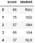
df = pd.DataFrame()
df["score"] = score_list
df.head()
-----------------------

#产生随机字符串,当成学生的名字
df['student'] = [pd.util.testing.rands(3) for i in range(20)]
df.head()
-------------------------------------
df['categoried'] = pd.cut(df["score"],bins,labels=["不及格","及格","良好","优秀"])
#给分箱的每个分数段取名
df.head()
-------------------------

数据分组:
import numpy as np
import pandas as pd
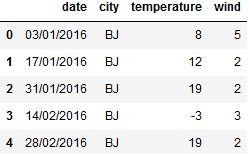
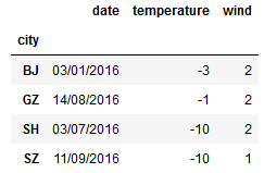
df = pd.read_clipboard()  #获取剪贴板数据
df.to_csv('city_weather.csv')  #保存成csv文件
df = pd.read_csv('city_weather.csv')
del df['Unnamed: 0']
df.head()
-------------------------------------
g = df.groupby(df['city']) #按city分组
g.groups
------------------------------------------
{'BJ': Int64Index([0, 1, 2, 3, 4, 5], dtype='int64'),
 'GZ': Int64Index([14, 15, 16, 17], dtype='int64'),
 'SH': Int64Index([6, 7, 8, 9, 10, 11, 12, 13], dtype='int64'),
 'SZ': Int64Index([18, 19], dtype='int64'}
df_bj = g.get_group('BJ') #获取BJ分组数据
df_bj
-------------------------------
df_bj.mean()  #取每个columns的平均值
g.max() #取每组每个colums的最大值
g.min()  #取每组每个colums的最小值
数据聚合:
import numpy as np
import pandas as pd
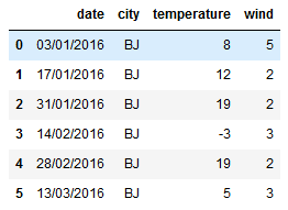
df = pd.read_csv('city_weather.csv')
g = df.groupby('city')
del df['Unnamed: 0']
print(df)
g.groups
-----------------

          date  city    temperature  wind
0   03/01/2016   BJ            8       5
1   17/01/2016   BJ           12       2
2   31/01/2016   BJ           19       2
3   14/02/2016   BJ           -3       3
4   28/02/2016   BJ           19       2
5   13/03/2016   BJ            5       3
6   27/03/2016   SH           -4       4
7   10/04/2016   SH           19       3
8   24/04/2016   SH           20       3
9   08/05/2016   SH           17       3
10  22/05/2016   SH            4       2
11  05/06/2016   SH          -10       4
12  19/06/2016   SH            0       5
13  03/07/2016   SH           -9       5
14  17/07/2016   GZ           10       2
15  31/07/2016   GZ           -1       5
16  14/08/2016   GZ            1       5
17  28/08/2016   GZ           25       4
18  11/09/2016   SZ           20       1
19  25/09/2016   SZ          -10       4

{'BJ': Int64Index([0, 1, 2, 3, 4, 5], dtype='int64'),
 'GZ': Int64Index([14, 15, 16, 17], dtype='int64'),
 'SH': Int64Index([6, 7, 8, 9, 10, 11, 12, 13], dtype='int64'),
 'SZ': Int64Index([18, 19], dtype='int64')}
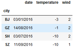
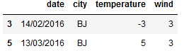
print(g.min())
print(g.agg('min')) #把每个分组最小的值聚合在一起
---------------------------------
#多条件分组聚合
g_new = df.groupby(['city','wind'])
g_new.groups
g_new.get_group(('BJ',3))
--------------------------------------
{('BJ', 2): Int64Index([1, 2, 4], dtype='int64'),
 ('BJ', 3): Int64Index([3, 5], dtype='int64'),
 ('BJ', 5): Int64Index([0], dtype='int64'),
 ('GZ', 2): Int64Index([14], dtype='int64'),
 ('GZ', 4): Int64Index([17], dtype='int64'),
 ('GZ', 5): Int64Index([15, 16], dtype='int64'),
 ('SH', 2): Int64Index([10], dtype='int64'),
 ('SH', 3): Int64Index([7, 8, 9], dtype='int64'),
 ('SH', 4): Int64Index([6, 11], dtype='int64'),
 ('SH', 5): Int64Index([12, 13], dtype='int64'),
 ('SZ', 1): Int64Index([18], dtype='int64'),
 ('SZ', 4): Int64Index([19], dtype='int64')}
透视表:
import numpy as np
import pandas as pd
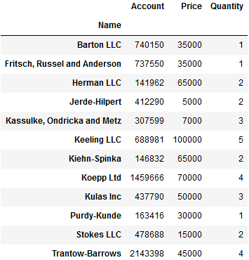
df = pd.read_excel('sales-funnel.xlsx') #读取数据文件
df
-------------------------------------------
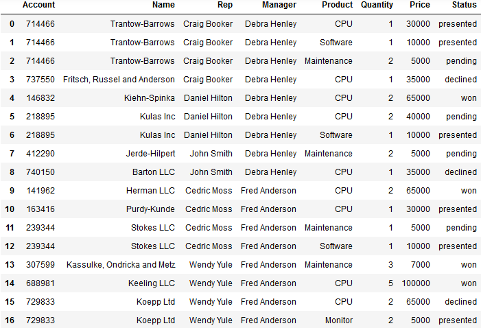
#透视表,默认以name为index将所有name可以计算的数据求平均值
pd.pivot_table(df,index='Name')
------------------------
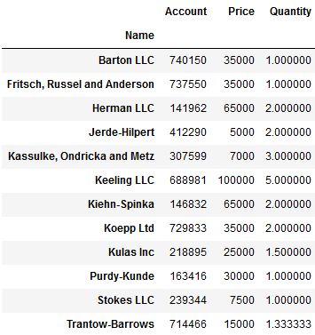
#求Name所有值的sum值透视表
pd.pivot_table(df,index=['Name'],aggfunc='sum')
-------------------------
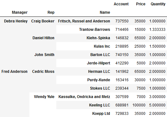
#取每个经理下 销售与客户的数据
pd.pivot_table(df,index=['Manager','Rep'])
--------------------------------
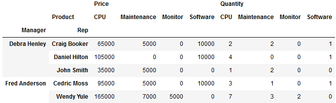
#统计经理下的销售卖了多少Product列里的物品,销售额多少,数量有多少
pd.pivot_table(df,index=['Manger','Rep'],
                     value=['Price','Quantity'],columns='Product',
                     fill_value=0,aggfunc='sum')   #fill_value是将表里的NAN填充成0
-----------------------------------------------
分组和透视表功能实战:
import numpy as np
import pandas as pd
df = pd.read_csv('2008.csv')
df.head()
-------------------------------
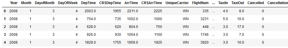
#取延误时间最长的10个航班
#排序函数,默认升序
#以ArrDelay列数值排序        降序            取十个数据
df.sort_values('ArrDelay',ascending=False)[:10][['DepTime','FlightNum',"ArrTime","Origin","Dest","ArrDelay"]]
-------------------------------------------------------
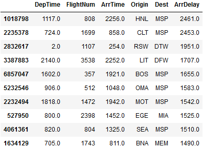
#查看没有延误的航班和延误航班的比例
print(df['Cancelled'].value_counts())
#查看没有延误的航班和延误航班的比例
print(df['Cancelled'].
matplotlib简单绘图-plot:
import numpy as np
import matplotlib.pyplot as plt
%matplotlib inline
#魔法方法,每次画完图不用show()自动就出来
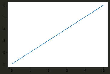
a = [1,2,3,4,5,6]
plt.plot(a)    #默认以a的index为x,a的值为y
-------------------------------
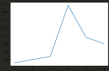
a = [1,2,3,4,5,6]
b = [4,5,6,22,12,10]
plt.plot(a,b)  #以a值为x,b值为y
-----------------------------
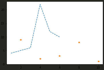
c = [10,8,6,4,2]
d = [1,8,3,2,9]
plt.plot(a,c,'--',c,d,'*')  #以a和c为x  b和d为y  ac用虚线,cd用星星
------------------------------
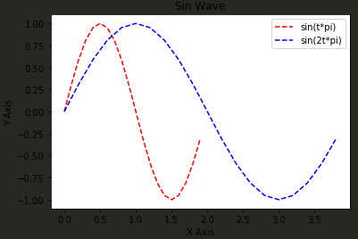
t = np.arange(0.0,2.0,0.1)
print(t)
s = np.sin(t*np.pi)
print(s)
----------------------------------
array([0. , 0.1, 0.2, 0.3, 0.4, 0.5, 0.6, 0.7, 0.8, 0.9, 1. , 1.1, 1.2,
1.3, 1.4, 1.5, 1.6, 1.7, 1.8, 1.9])

=============

[ 0.00000000e+00,  3.09016994e-01,  5.87785252e-01,  8.09016994e-01,
  9.51056516e-01,  1.00000000e+00,  9.51056516e-01,  8.09016994e-01,
  5.87785252e-01,  3.09016994e-01,  1.22464680e-16, -3.09016994e-01,
 -5.87785252e-01, -8.09016994e-01, -9.51056516e-01, -1.00000000e+00,
 -9.51056516e-01, -8.09016994e-01, -5.87785252e-01, -3.09016994e-01]
plt.plot(t,s,'r--',label='sin(t*pi)')  #用红色虚线t为x s为y,label设置显示图例
plt.plot(t*2,s,'b--',label='sin(2t*pi)')
plt.xlabel('X Axis')   #给x线取名
plt.xlabel('Y Axis')      #给y线取名
plt.title('Sin Wave')    #图表名
plt.legend()              #显示label
----------------------------------
matplotlib绘子图-subplot:
import numpy as np
import matplotlib.pyplot as plt
%matplotlib inline
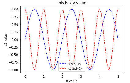
x = np.linspace(0.0,5.0)   #以0开始到5.0取50个数
y1 = np.sin(np.pi*x)
y2 = np.cos(np.pi*x*2)

plt.plot(x,y1,'b--',label='sin(pi*x)')
plt.plot(x,y2,'r--',label='cos(pi*2x)')
plt.ylabel('y value')
plt.xlabel('x value')
plt.legend()
--------------------------------------------------
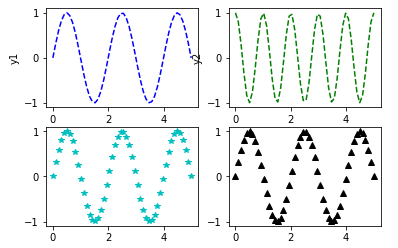
plt.subplot(2,2,1)   #将图画在2*2个窗口的第一个窗口  可写成221,也是同样效果
plt.plot(x,y1,'b--')
plt,ylabel('y1')

plt.subplot(222)
plt.plot(x,y2,'r--')
plt,ylabel('y2')

plt.subplot(223)
plt.plot(x,y1,'c*')

plt.subplot(224)
plt.plot(x,y1,'k^')
-----------------------------------
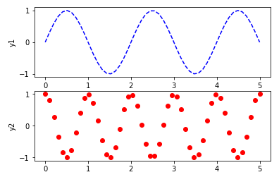
plt.subplot(211)
plt.plot(x,y1,'b--')
plt.ylabel('y1')

plt.subplot(212)
plt.plot(x,y2,'ro')   #红色点状
plt.ylabel('y2')

plt.xlabel('x')
-------------------------------------
import numpy as np
import pandas as pd
import matplotlib.pyplot as plt
%matplotlib inline
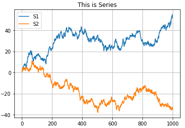
s1 = pd.Series(np.random.randn(1000)).cumsum()
#cumsum为累计求和,即(((1+2)+3)+4).....
s1 = pd.Series(np.random.randn(1000)).cumsum()
s1.plot(kind='line',label='S1',title='Thie is Series')  #Series和DataFrame自带plot
s2.plot(label='S2',grid=True)  #grid是否显示网格
plt.legend()
-----------------------------------
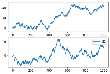
#使用plt的plot来画
figure,ax = plt.subplots(2,1)
ax[0].plot(s1,label='S1')
ax[1].plot(s2,label='S2')
plt.legend()
----------------------------
import numpy as np
import pandas as pd
import matplotlib.pyplot as plt
%matplotlib inline
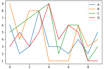
df = pd.DataFrame(np.random.randint(1,10,40).reshape(10,4),
                            columns=['A','B','C','D'])
#创建40个1-10的随机数,将其转为10行4列
df
-----------------------------------------

#使用DataFrame自带的plot
df.plot()
-------------------
#使用plt的plot
plt.plot(df['A'],label='A')
plt.plot(df['B'],label='B')
plt.plot(df['C'],label='C')
plt.plot(df['D'],label='D')
plt.legend()
----------------------
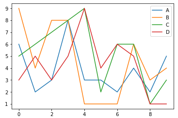
总结:特定情况下使用DataFrame和Series自带的plot更方便
import numpy as np
import pandas as pd
import matplotlib.pyplot as plt
%matplotlib inline
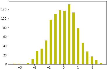
#直方图
s = pd.Series(np.random.randn(1000))
plt.hist(s,bins=20,rwidth=0.5,color='y')
#hist使用直方图,bins设置20个区间,rwidth是柱子的宽度,color是柱子的颜色
-----------------------------------------
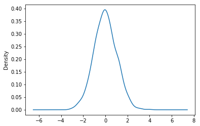
#密度图
s.plot(kind='kde')
---------------------
Seaborn画图:
import numpy as np
import pandas as pd
import matplotlib.pyplot as plt
import seaborn as sns
%matplotlib inline
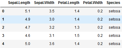
iris = pd.read_csv(r"iris.csv")
del iris['Unnamed: 0']
iris.head()
#sepal 花萼  petal花瓣   species 种类
----------------------------------------
iris.Species.unique()  #将Species去重,查看有几个种类
----------------------------
['setosa', 'versicolor', 'virginica']
#用zip给每种花定义一个颜色
color_map = dict(zip(iris.Species.unique(),['blue','green','red']))
color_map
----------------------
{'setosa': 'blue', 'versicolor': 'green', 'virginica': 'red'}
#将iris分组后进行画图
for species,group in iris.groupby('Species'):   #以Species分组后的数据进行for循环
    plt.scatter(group['Petal.Width'],group['Sepal.Width'],
                    color = color_map[species],  #用species取出来的种类在color_map取颜色
                    alpha=0.3,  #透明度
                    edgecolor='black',  #每个点的边框
                    label=species)
    plt.legend(frameon=True,title='Species')  #frameon 是否开启label标签边框
    plt.xlabel('Petal.Width')
    plt.ylabel('Sepal.Width')
----------------------------

#使用Seaborn来画
sns.lmplot('Petal.Width','Sepal.Width',iris,hue='Species',fit_reg=False)
#hue会自动区分Species的种类然后自动配色和label,fit_reg是否打开回归线
----------------------------------------------

Seaborn的密度图
s1 = pd.Series(np.random.randn(1000))
sns.distplot(s1,bins=20,hist=True,kde=True,rut=True)
#hist是否开启直方图,kde是否开启数据线,rut是否开启密度图
-----------------------------

sns.heatmap(data,annot=True,fmt='d')
#热力图  annot是否在每个格子里显示数字  fmt显示的数据类型 d整数 .2f是2位小数点的浮点型

sns.barplot(x=x轴放什么数据,y=y轴放什么数据) #sns柱状图
股票市场分析:
import numpy as np
import pandas as pd

import pandas_datareader as pdr #读取数据的模块

import matplotlib.pylab as plt  #图形可视化
import seaborn as sns
%matplotlib inline
#魔法命令,可以让图形不用show()命令就能出来

from datetime import datetime
start = datetime(2015,9,20) #获取阿里巴巴和亚马逊从2015-9-20开始的数据 alibaba = pdr.get_data_yahoo('BABA',start=start) amazon = pdr.get_data_yahoo('AMZN',start=start)
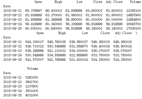
print(alibaba.head())
print(amazon.head())
--------------------------------------------------
#保存数据
alibaba.to_csv('BABA.csv')
amazon.to_csv('AMZN.csv')
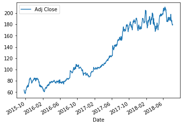
alibaba['Adj Close'].plot(legend=True) #用图形显示阿里巴巴Adj Close项的走势
#Series和DataFrame都自带plot,legend是否显示label
--------------------------------------------
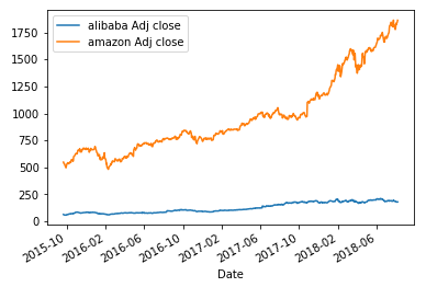
#对比两只股票的Adj Close
alibaba['Adj Close'].plot(legend=True,label='alibaba Adj close')
alibaba['Adj Close'].plot(legend=True,label='alibaba Adj close')
-----------------------------------
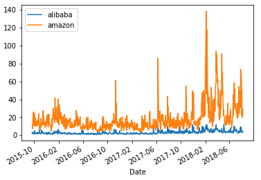
#将股票每日最大波动添加到新列  最高值-最低值
alibaba['high-low'] = alibaba['High'] - alibaba['Low']
amazon['high-low'] = amazon['High'] - amazon['Low']
print(alibaba.head())
print(amazon.head())
-------------------------------
                 Open       High        Low      Close  Adj Close    Volume  \
Date
2015-09-21  65.379997  66.400002  62.959999  63.900002  63.900002  22355100
2015-09-22  62.939999  63.270000  61.580002  61.900002  61.900002  14897900
2015-09-23  61.959999  62.299999  59.680000  60.000000  60.000000  22684600
2015-09-24  59.419998  60.340000  58.209999  59.919998  59.919998  20645700
2015-09-25  60.630001  60.840000  58.919998  59.240002  59.240002  17009100

            high-low
Date
2015-09-21  3.440003
2015-09-22  1.689998
2015-09-23  2.619999
2015-09-24  2.130001
2015-09-25  1.920002
                  Open        High         Low       Close   Adj Close  \
Date
2015-09-21  544.330017  549.780029  539.590027  548.390015  548.390015
2015-09-22  539.710022  543.549988  532.659973  538.400024  538.400024
2015-09-23  538.299988  541.210022  534.000000  536.070007  536.070007
2015-09-24  530.549988  534.559998  522.869995  533.750000  533.750000
2015-09-25  542.570007  542.799988  521.400024  524.250000  524.250000

             Volume   high-low
Date
2015-09-21  3283300  10.190002
2015-09-22  3841700  10.890015
2015-09-23  2237600   7.210022
2015-09-24  3501000  11.690003
2015-09-25  4031000  21.399964
#用波动值画图
alibaba['high-low'].plot(label='alibaba',legend=True)
amazon['high-low'].plot(label='amazon',legend=True)
---------------------------------------
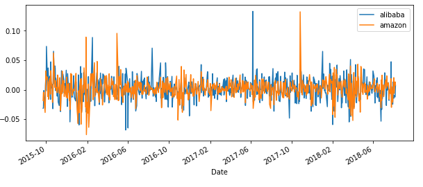
#计算两个交易日间最后操作收盘价的波动
alibaba['dialy-return'] = alibaba['Adj Close'].pct_change()
#pct_change() 计算相邻两行之间数值的变化
amazon['dialy-return'] = alibaba['Adj Close'].pct_change()
alibaba['dialy-return'].plot(figsize=(10,4),legend=True,label='alibaba')
#figsize调整画布大小
amazon['dialy-return'].plot(figsize=(10,4),legend=True,label='amazon')
----------------------------------------------------------------------------
alibaba['dialy-return'].plot(kind='hist')  #直方图

sns.distplot(amazon['dialy-return'].dropna(),bins=100,color='blue',
             label='amazon',rug=True)
#用seabron画的密度图,因为dialy-return第一行是Nan,所以要dropnan
#rug是开启密度图形
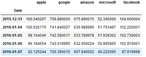
top_tech_df = pd.read_csv('top5.csv',index_col='Date')
#读取文件数据,以Date作为index
top_tech_df.head()
-----------------------------------
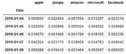
top_tech_dr = top_tech_df.pct_change()  #计算Adj close波动
top_tech_dr.dropna().head()
------------------------------------
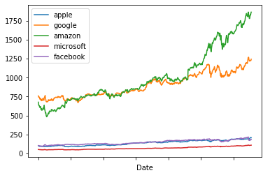
top_tech_df.plot()
--------------------------
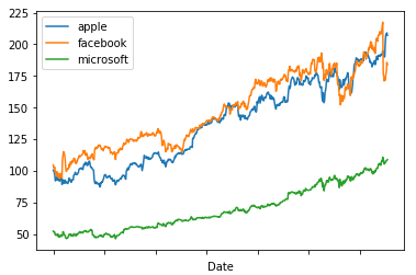
top_tech_df[['apple','facebook','microsoft']].plot()
#只取3家公司的股票图
----------------------------
#pairplot让所有columns和另外4个任意一个columns画出散点图
#因为top_tech_dr的第一行都是NAN,所以要drop掉
sns.pairplot(top_tech_dr.dropna())
--------------------------------------


 浙公网安备 33010602011771号