不同可视化要求的代码

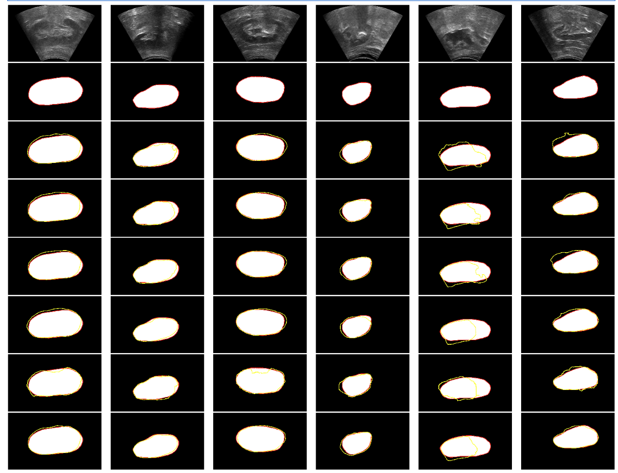
要求1.论文写作中不同模型输出对比

• 需要自己提供，输入图像、以及对应mask还有不同模型的预测结果。

# 可视化图像、mask、不同模型的输出
import matplotlib.pyplot as plt
import cv2
from pathlib import Path
import os
from skimage import io, measure
import numpy as np

# network_name = ["CPFNet", "Deep", "Deepplus", "FPN", "LinkNet", "SegNet", "UNet", "swin", "PSPNet"]
network_name = ["CPFNet", "Deep", "Deepplus", "FPN", "swin", "PSPNet"]


# case = "wdus0000"
cases = ["wdus0000", "wdus0001", "wdus0007", "wdus0015", "wdus0016", "wdus0027",]
direction = "l1_120"
case_begin_index = 0
# case_begin_indexs = [0, 1]

image_root_path = r"/home/chaochen/Rashid/task02/Trainset/images/"
mask_root_path = r"/home/chaochen/Rashid/task02/Trainset/masks/"
output_root_path = r"/home/chaochen/Rashid/task02/imgAndcode/outall"
seg_root_path = r"/home/chaochen/Rashid/task02/imgAndcode/"

linewidth = 5


image_coutour_out = os.path.join(output_root_path, "image", rf"{case}/{direction}/{case_begin_index}_image.png")
mask_coutour_out = os.path.join(output_root_path, "mask", rf"{case}/{direction}/{case_begin_index}_mask.png")

Path(os.path.join(output_root_path, rf"mask/{case}/{direction}")).mkdir(parents=True, exist_ok=True)
Path(os.path.join(output_root_path, rf"image/{case}/{direction}")).mkdir(parents=True, exist_ok=True)

# 每一列第一行是输入图像，第二行是mask，之后每行分别是不同模型的输出

fig, axs = plt.subplots(8, 6, figsize=(80, 60), dpi=300)
for col_index in range(6):
    # case_begin_index = case_begin_indexs[col_index]
    case = cases[col_index]
    image_path = os.path.join(image_root_path, case, direction, f"{case_begin_index}.png")
    mask_path = os.path.join(mask_root_path, case, direction, f"{case_begin_index}.png")
    

    img = io.imread(image_path)
    mask = io.imread(mask_path)
    # plot image
    axs[0, col_index].imshow(img, cmap='gray')
    axs[0, col_index].axis("off")
    axs[0, col_index]
    # plot mask
    mask_contour = measure.find_contours(mask)[0]
    axs[1, col_index].imshow(mask, cmap='gray')
    axs[1, col_index].plot(mask_contour[:, 1], mask_contour[:, 0], linewidth=linewidth, color='red')
    axs[1, col_index].axis("off")


    for index, network in enumerate(network_name):
        # network = network_name[index-2]
        pred_path = os.path.join(seg_root_path, network, "test_result", case, direction, f"{case_begin_index}.png")
        pred_coutour_out = os.path.join(output_root_path, rf"{network}/{case}/{direction}/{case_begin_index}_pred.png")
        Path(os.path.join(output_root_path, rf"{network}/{case}/{direction}")).mkdir(parents=True, exist_ok=True)

        pred = io.imread(pred_path)
        mask = io.imread(mask_path)

        pred_coutour = measure.find_contours(pred)[0]
        mask_coutour = measure.find_contours(mask)[0]

        # 红色表示gt
        # 画mask 边界
        axs[index+2, col_index].plot(mask_coutour[:, 1], mask_coutour[:, 0], linewidth=linewidth, color='red')
        # # 显示mask
        # axs[index+2].imshow(mask, cmap="gray")
        # # 保存
        # axs[index+2].savefig(mask_coutour_out, bbox_inches='tight', pad_inches=0)

        # 黄色表示预测的mask
        # 画预测结果的边界
        axs[index+2, col_index].plot(pred_coutour[:, 1], pred_coutour[:, 0], linewidth=linewidth, color='yellow')
        # 显示mask
        axs[index+2, col_index].imshow(mask, cmap="gray")
        axs[index+2, col_index].axis("off")
        # axs[index+2].savefig(pred_coutour_out, bbox_inches='tight', pad_inches=0)
        # axs[index+2].clf()

plt.tight_layout()
plt.savefig('wdus0000_l1_120.png', dpi=300)
plt.show()

输出结果显示：

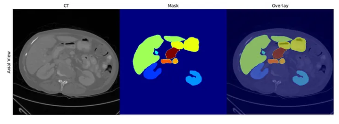
要求2. 一行分别显示3D CT image(灰色)， mask（标签不同色），image和mask放在一起

• 准备CT image 和mask 张量（h w D）

f, axarr = plt.subplots(1,3,figsize=(15,15))
axarr[0].imshow(np.squeeze(image[100, :, :]), cmap='gray',origin='lower');
axarr[0].set_ylabel('Axial View',fontsize=14)
axarr[0].set_xticks([])
axarr[0].set_yticks([])
axarr[0].set_title('CT',fontsize=14)

axarr[1].imshow(np.squeeze(mask[100, :, :]), cmap='jet',origin='lower');
axarr[1].axis('off')
axarr[1].set_title('Mask',fontsize=14)

axarr[2].imshow(np.squeeze(image[100, :, :]), cmap='gray',alpha=1,origin='lower');
axarr[2].imshow(np.squeeze(mask[100, :, :]),cmap='jet',alpha=0.5,origin='lower');
axarr[2].axis('off')
axarr[2].set_title('Overlay',fontsize=14)
plt.tight_layout()
plt.subplots_adjust(wspace=0, hspace=0)

• 效果展示