机器学习基石 之 机器学习实现与可行性（Feasibility）分析

什么是机器学习（Machine Learing）

首先我们应该弄清楚什么是学习。

learning: acquiring skill with experience accumulated from observations

machine learning: acquiring skill with experience accumulated/computed from data

相较于学习而言机器学习是通过观察数据从而获得技能。

具体来说：skill便是在某些性能指标（improving some performance measure）。所以说机器学习的定义可以具体为：

machine learning：improving some performance measure with experience computed from data

但是同时由于机器学习又经常用于为复杂问题构建解决方案，即可以用于复杂系统的构建，所以机器学习的另一种定义为：

machine learning：an alternative route to build complicated systems

当然如此工具，有三个关键点（Key Essence of Machine Learning）：

1. exists some ‘underlying pattern’ to be learned
   —so ‘performance measure’ can be improved
2. but no programmable (easy) definition
   —so ‘ML’ is needed
3. somehow there is data about the pattern
   —so ML has some ‘inputs’ to learn from

其中第一点和第三点是进行机器学习的前提条件，第二点是为防止机器学习滥用，即简单&可人为处理的问题不需要机器学习。

英语单词学习：
navigate 使通过，oriented 标定方向的，scale 规模衡量，poisoning 中毒，properly 适当非常，likeliness 可能

本课总结：Machine-Learing is everywhere ❗

学习问题的基本形式 （Formalize the Learning Problem）

基本符号（Basic Notations）

属性（attribute）或特征（feature）：反映事件或对象在某方面的表现或性质的事项。属性张成的空间又叫样本空间（sample space）或属性空间（attribute space）: \(\mathcal{X}\)。

示例（instance）或样本（sample）或输入（input）： \(\boldsymbol{x}_{i}=\left(x_{i 1}x_{i 2} ; \ldots ; x_{i d} \right)\)，是 \(d\) 维样本空间 \(\mathcal{X}\) 中的一个向量（特征向量），其中\(x_{ij}\)是\(x_i\)在第\(j\)个属性上的取值， \(d\) 称为样本 \(x_{i}\)的维数(dimensionality)。

标记（label）或输出（output）：\(y_i\)，关于示例\(x_i\)结果的信息。标记张成的空间又叫标记空间（label space) : \(\mathcal{Y}\)。

样例（example）：\(\left(x_{i}, y_{i}\right)\)，拥有标记的示例。

目标函数（target function）：未知的需要学习的模式（unknown pattern to be learned)，前面提及到的skill的终极模式，即属性和标记之间的真实映射关系：\(f(x) = y\)。

数据集（data set）：一组关于某事件或对象的记录（样例）的集合，数学表示为\(D=\left\{\boldsymbol{x}_{1}, \boldsymbol{x}_{2}, \ldots, \boldsymbol{x}_{m}\right\}\)，分为训练集(training set)和测试集(test set)。

模型（model）或假设（hypothesis）：学得模型对应了关于数据的某种潜在的规律，通过对数据观察学习到的属性和标记之间的近似映射关系：\(h:\mathcal{X} \rightarrow \mathcal{Y}\)；这种潜在规律自身，则称为“真相”或“真实”（ground-truth），学习过程就是为了找出或逼近真相。有时将模型称为“学习器”（learner），可看作学习算法在给定数据和参数空间上的实例化。所有的\(h\)组成了假设函数集\(H\)，其中伪最优的假设函数（‘best’ hypothesis)将被叫做 \(g\)。

学习（learning）或训练（training）：从数据中学得模型的过程，这个过程通过执行某个学习算法（learning algorithm）\(\mathcal{A}\)来完成。

测试（testing）：学得模型后，使用其进行预测的过程，被预测的样本称为测试样本（testing sample）。

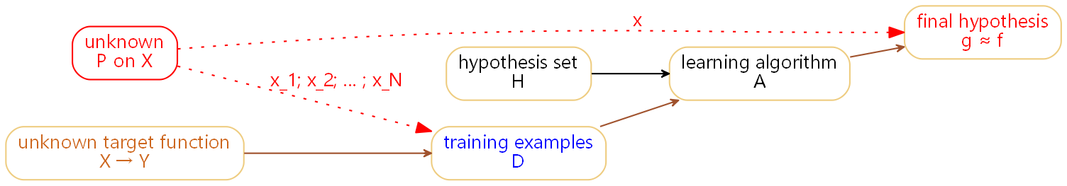
学习流程（Learning Flow）

上图便是机器学习的基本流程图。其中learning algorithm \(\mathcal{A}\)便是在所有的假设函数函数选取出 \(g\)（‘best’ hypothesis) (\(\mathcal{A}\) takes \(\mathcal{D}\) and \(\mathcal{H}\) to get \(\mathcal{g}\))。所以该流程图又可画为：

从该流程图出发可以获得机器学习的最终定义为：从数据出发计算出接近于目标函数 \(f\) 的伪最优假设函数 \(g\) (use data to approximate target)，即\(g \approx f\)。

机器学习与数据挖掘/人工智能/统计学

数据挖掘/人工智能/统计学的定义如下

Data Mining ：use (huge) data to find property that is interesting.

Artificial Intelligence ：compute something that shows intelligent behavior

Statistics ：use data to make inference about an unknown process

简单来说数据挖掘虽然有时跟机器学习很相似，但是在实际中分析却很不同，当然数据挖掘有时对机器学习很有帮助，机器学习是实现人工智能的一种方法，而统计学有许多工具用于实现机器学习的方法。

如何实现二分类（Binary Classification）

感知机（Perceptron)

以是否发放信用卡为例，在生活中最简单的方式便是根据一个人的属性：年龄，参加工作的时间，薪资和当前的信誉度对一个人进行评判。而感知机则是利用全部属性的线性组合进行计算是否发卡的分数，而每个属性的系数则是每个属性的所占比重。

property	value
age	23 years
annual salary	NTD 1,000,000
year in job	0.5 year
current debt	200,000

这里属性就是前面所提到的特征features of customer构成这个人的特征向量→ \(\mathbf{x}=\left(x_{1}, x_{2}, \cdots, x_{d}\right)\) ，而每个属性或特征所占的比重weight构成这个人的比重向量 → \(\mathbf{w}=\left(w_{1}, w_{2}, \cdots, w_{d}\right)\)。这样便可以根据两者计算分数，进而使用阈值判断决定是否进行发卡。

\[\text { score } = \sum_{i=1}^{d} w_{i} x_{i}\\ \begin{array}{l}\text{approve credit if} \quad & \text { score } > \text{threshold}\\ \text{deny credit if} \quad & \text { score } < \text{threshold}\end{array} \]

那么可以将上述问题总结为一个线性假设函数（linear formula） \(h \in \mathcal{H}\)：

\[h(\mathbf{x})=\operatorname{sign}\left(\left(\sum_{i=1}^{d} w_{i} x_{i}\right)-\text { threshold }\right) \]

这里的sign(x)表示的是取变量符号的函数，当x小于零取-1，当x大于零取1。

 那么假设函数的输出空间即标记空间可以表示为$\mathcal{Y}:\{+1(\text { good }),-1(\text { bad })\}, 0 \text{ ignored}$ 。而这便是感知机的基本数学形式，而感知机名字的由来是由于历史原因。

为了简化公式这里令\(w_0 = 1 , x_0 = \text{threshold}\)，那么可以将上述的两个特征向量和比重向量改写为 \(\mathbf{x}=\left(x_{0},x_{1}, x_{2}, \cdots, x_{d}\right)\) ， \(\mathbf{w}=\left(w_{0},w_{1}, w_{2}, \cdots, w_{d}\right)\)。那么该假设函数可以改写为：

\[h(\mathbf{x})=\operatorname{sign}\left(\mathbf{w}^{T}\mathbf{x}\right) \]

那么感知机在二维空间 \(\mathbb{R}^{2}\) 可写为：

\[h(\mathbf{x})=\operatorname{sign}\left(w_{0}+w_{1} x_{1}+w_{2} x_{2}\right) \]

其表现如下图所示，其中标签y的表现形式为：o (+1), × (-1)，而上述假设函数的表现形式便是lines (or hyperplanes in \(\mathbb{R}^{2}\) ，二维空间的超平面)，而理想状态下正负样本则分别在其两侧（positive on one side of a line, negative on the other side）。

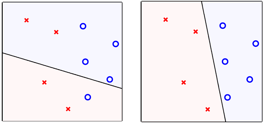
可见感知机便是简单的线性二分类器。

感知机学习算法（PLA）

理论分析

感知机模型已经建立，那么根据机器学习流程图，便需要一个学习算法（Learning Algorithm) \(\mathcal{A}\) 选取假设函数使得 \(g \approx f \text{ on } \mathcal{D}\) ，理想状态下是\(g(\mathbf{x}_n)=f(\mathbf{x}_n)=y_n\)。但是问题是假设函数集\(\mathcal{H}\)是无穷大（infinite size）的。

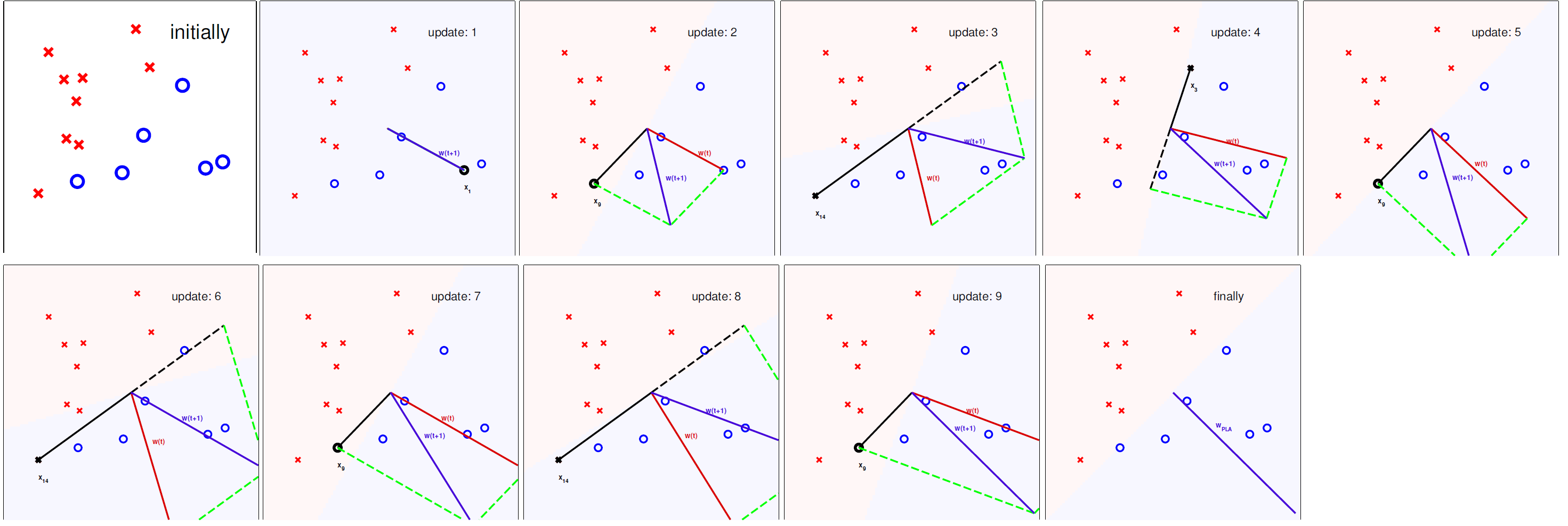
一个思路是从一个初始假设函数 \(g_0\) （或\(\mathbf{w}_0\)，因为由于感知机本身的特点，\(\mathbf{w}_i\)便可以代表\(\mathbf{g}_i\)）开始迭代，并且纠正（correct）该假设函数在 \(\mathcal{D}\) 上犯得分类错误，而感知机学习算法（Perceptron Learning Algorithm）便是如此实现的。

PLA实现步骤如下：

For \(t=0,1, \ldots\)

• find a mistake of \(\mathbf{w}_{t}\) called \(\left(\mathbf{x}_{n(t)}, y_{n(t)}\right)\)

\[\operatorname{sign}\left(\mathbf{w}_{t}^{T} \mathbf{x}_{n(t)}\right) \neq y_{n(t)} \]

• (try to) correct the mistake by

\[\mathbf{w}_{t+1} \leftarrow \mathbf{w}_{t}+y_{n(t)} \mathbf{x}_{n(t)} \]

until no more mistakes return last \(\mathbf{w}\) (called \(\mathbf{w}_{\mathrm{PLA}}\) ) as \(g\).

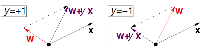
将向量相加操作在二维平面可表示为：

知识回顾：

• 向量的叉积：\(a \times b = |a| |b| \sin (a,b)\)
• 向量的点积：\(a \cdot b = |a| |b| \sin (a,b) = a^{T}b\)

所以当\(y_n > 0, \mathbf{w}_n^{T}\mathbf{x}_n < 0\)时想使\(\mathbf{w}_n^{T}\mathbf{x}_n\)向\(y_n\)逼近，那么\(\mathbf{w}_n\) 和 \(\mathbf{x}_n\) 的夹角应该由钝角转为锐角，即旋转\(\mathbf{w}_n\) 向 \(\mathbf{x}_n\) 靠近，那么使用第二步公式便可以实现，反之同理可证。

引用名言：

知错能改，善莫大焉。

A fault confessed is half redressed. 😉

可以看出该算法可以实现权重的学习，并且使得该分类器可以实现正负样本的分类（正负样本分别位于超平面的一侧）。

具体实现

之前有提到直到不犯错误时停止算法运行，这里提出在一个循环周期内不犯错误那么便认为全部分类正确，所以便有了Cyclic PLA（循环感知机学习算法）。

Cyclic PLA实现步骤如下：

For \(t=0,1, \ldots\)

• find a mistake of \(\mathbf{w}_{t}\) called \(\left(\mathbf{x}_{n(t)}, y_{n(t)}\right)\)

\[\operatorname{sign}\left(\mathbf{w}_{t}^{T} \mathbf{x}_{n(t)}\right) \neq y_{n(t)} \]

• (try to) correct the mistake by

\[\mathbf{w}_{t+1} \leftarrow \mathbf{w}_{t}+y_{n(t)} \mathbf{x}_{n(t)} \]

until a full cycle of not encountering mistakes.

这里与PLA不同的地方是结束条件是一个循环周期内无误差，至于在循环周期内是纯粹的遍历一个周期\((1, \cdots ,N)\)或者是随机遍历一个周期（precomputed random cycle）便可以视情况而定。

由于PLA的实现方式是需要全部的样本均分类正确无误。这样导致PLA可能需要执行较长的时间，才能完成，并且样本中不允许有噪声。这样的条件是很苛刻的，所以在实际运用中常常以足够多的纠正次数（‘enough’ corrections），作为PLA变体的停止条件。

可行性分析 \(E_{\text{in}} \approx 0\)

PLA的可行性分析实际上就是分析PLA算法是否最终会停止。

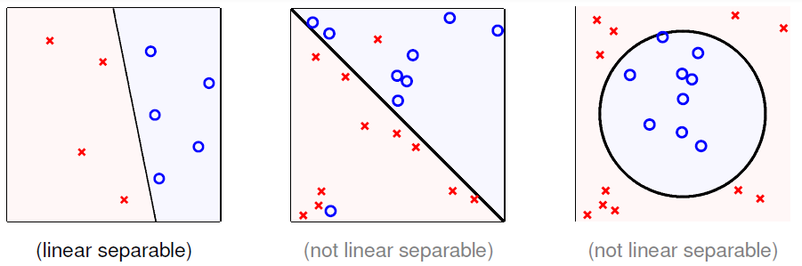
下面先了解一下线性可分，其定义如下

if PLA halts (i.e. no more mistakes)， (necessary condition) \(\mathcal{D}\) allows some \(\mathbf{w}\) to make no mistake，call such \(\mathcal{D}\) linear separable.

如果PLA停止，那么必要条件是存在超平面 \(h_f\)（由\(\mathbf{w}_f\)构成的假设函数，\(h_{f}(\mathbf{x}_n)=\operatorname{sign}\left(\mathbf{w}_{f}^{T} \mathbf{x}_{n}\right) = y_{n}\)） 可以将数据集 \(\mathcal{D}\) 进行无误切分，那么便说 \(\mathcal{D}\) 是线性可分的。

例图如下：

假设数据是线性可分的，即存在\(\mathbf{w}_f\)用于构造分割的超平面。那么\(\mathbf{w}_f\)有以下两个性质：

由于每一个 \(\mathrm{x}_{n}\) 都被正确的被线分开（correctly away from line），所以有：

\[y_{n(t)} \mathbf{w}_{f}^{T} \mathbf{x}_{n(t)} \geq \min _{n} y_{n} \mathbf{w}_{f}^{T} \mathbf{x}_{n}>0 \]

同时根据每一个分类错误的样本 \(\left(\mathbf{x}_{n(t)}, y_{n(t)}\right)\)对\(\mathbf{w}_{t}\)进行更新都会使得\(\mathbf{w}_{f}^{T} \mathbf{w}_{t} \uparrow\)，即：

\[\begin{aligned} \mathbf{w}_{f}^{T} \mathbf{w}_{t+1} &=\mathbf{w}_{f}^{T}\left(\mathbf{w}_{t}+y_{n(t)} \mathbf{x}_{n(t)}\right) \\ & \geq \mathbf{w}_{f}^{T} \mathbf{w}_{t}+\min _{n} y_{n} \mathbf{w}_{f}^{T} \mathbf{x}_{n} \\ &>\mathbf{w}_{f}^{T} \mathbf{w}_{t}+0 \end{aligned} \]

从上述公式可以进一步推导有：

\[\begin{aligned} \mathbf{w}_{f}^{T} \mathbf{w}_{t} & \geq \mathbf{w}_{f}^{T} \mathbf{w}_{t}+\min _{n} y_{n} \mathbf{w}_{f}^{T} \mathbf{x}_{n} \\ ^{\text{recurrence } \Rightarrow} &\geq \mathbf{w}_{f}^{T} \mathbf{w}_{0}+T \min _{n} y_{n} \mathbf{w}_{f}^{T} \mathbf{x}_{n} \\ ^{{\mathbf{w}_0=0} \text{ } \Rightarrow} &\geq T \min _{n} y_{n} \mathbf{w}_{f}^{T} \mathbf{x}_{n} \end{aligned} \]

即：\(\mathbf{w}_{f}^{T} \mathbf{w}_{t} \geq T \min _{n} y_{n} \mathbf{w}_{f}^{T} \mathbf{x}_{n}\)。

前文中推导过PLA的更新策略是会使得 \(\mathbf{w}_{t}\) 向 \(\mathbf{w}_{f}\) 不断逼近的，即两者的夹角不断趋近于0️⃣，余弦值趋近于1️⃣，用向量表示就是：

\[\frac{\mathbf{w}_{f}^{T}}{\left\|\mathbf{w}_{f}\right\|} \frac{\mathbf{w}_{T}}{\left\|\mathbf{w}_{T}\right\|} \rightarrow 1 \]

所以说在不考虑两个向量长度(模) 的时候，上述所推可以大概理解为两个向量是不断逼近的。

下面进行\(\left\|\mathbf{w}_{t}\right\|^{2}\)的分析（因为\(\left\|\mathbf{w}_{f}\right\|^{2}\)为常值无需分析）：

\[\begin{aligned} \left\|\mathbf{w}_{t+1}\right\|^{2} &=\left\|\mathbf{w}_{t}+y_{n(t)} \mathbf{x}_{n(t)}\right\|^{2} \\ &=\left\|\mathbf{w}_{t}\right\|^{2}+2 y_{n(t)} \mathbf{w}_{t}^{T} \mathbf{x}_{n(t)}+\left\|y_{n(t)} \mathbf{x}_{n(t)}\right\|^{2} \\ ^{\mathbf{w}_t \text{ changed } \Leftrightarrow \operatorname{sign}\left(\mathbf{w}_{t}^{T} \mathbf{x}_{n(t)}\right) \neq y_{n(t)} \Leftrightarrow y_{n(t)} \mathbf{w}_{t}^{T} \mathbf{x}_{n(t)} \leq 0 \text{ } \Rightarrow} & \leq\left\|\mathbf{w}_{t}\right\|^{2}+0+\left\|y_{n(t)} \mathbf{x}_{n(t)}\right\|^{2} \\ & \leq\left\|\mathbf{w}_{t}\right\|^{2}+\max _{n}\left\|y_{n} \mathbf{x}_{n}\right\|^{2} \end{aligned} \]

可以看出\(\left\|\mathbf{w}_{t}\right\|^{2}\) 成长速度有限，且每次的涨幅由 'longest' \(\mathbf{x}_{n}\) 限制，从上述公式可以进一步推导有：

\[\begin{aligned} \left\|\mathbf{w}_{t}\right\|^{2} & \leq\left\|\mathbf{w}_{t-1}\right\|^{2}+\max _{n}\left\|y_{n} \mathbf{x}_{n}\right\|^{2}\\ ^{\text{recurrence } \Rightarrow} &\leq \left\|\mathbf{w}_{0}\right\|^{2}+ T \max _{n}\left\|y_{n} \mathbf{x}_{n}\right\|^{2}\\ ^{{\mathbf{w}_0=0} \text{ } \Rightarrow}&\leq T \max _{n}\left\|y_{n} \mathbf{x}_{n}\right\|^{2}\\ \end{aligned} \]

那么有上述所推可以得出：

\[\begin{aligned} \frac{\mathbf{w}_{f}^{T}}{\left\|\mathbf{w}_{f}\right\|} \frac{\mathbf{w}_{T}}{\left\|\mathbf{w}_{T}\right\|} &\geq \frac{ T {\mathop {\min }\limits_n } y_{n} \mathbf{w}_{f}^{T} \mathbf{x}_{n} }{\left\|\mathbf{w}_{f}\right\| \cdot \sqrt{T {\mathop {\max }\limits_n }\left\|y_{n} \mathbf{x}_{n}\right\|^{2}}}\\ &\geq \frac{T {\mathop {\min }\limits_n } y_{n} \mathbf{w}_{f}^{T} \mathbf{x}_{n}}{\left\|\mathbf{w}_{f}\right\| \cdot \sqrt{T} {\mathop {\max }\limits_n } \left\|y_{n} \mathbf{x}_{n}\right\|}\\ &\geq \sqrt{T}\frac{ {\mathop {\min }\limits_n } y_{n} \mathbf{w}_{f}^{T} \mathbf{x}_{n}}{\left\|\mathbf{w}_{f}\right\| \cdot {\mathop {\max }\limits_n } \left\|y_{n} \mathbf{x}_{n}\right\|}\\ &\geq \sqrt{T} \cdot \text{constant} \end{aligned} \]

又因为 \(\frac{\mathbf{w}_{f}^{T}}{\left\|\mathbf{w}_{f}\right\|} \frac{\mathbf{w}_{T}}{\left\|\mathbf{w}_{T}\right\|} \leq 1\) ，所以 \(\sqrt{T}\) 为有限值，即循环次数 \(T\) 有限，PLA一定在有限时间内停止。

所以可以总结上述推导为：

当数据线性可分且通过错误进行修正时：

• \(\mathbf{w}_{t}\) 和 \(\mathbf{w}_{f}\) 的内积增长较快，但 \(\mathbf{w}_{t}\) 的长度增长较缓。
• \(\mathbf{w}_{t}\) （PLA所获取的超平面法向量）不断向 \(\mathbf{w}_{f} \Rightarrow\) halts 逼近

口袋算法（Pocket Algorithm）

口袋算法（Pocket Algorithm）：PLA算法的变体，每轮循环均保留最佳权值向量在口袋中（keeping best weights in pocket）。

口袋算法实现步骤如下：

initialize pocket weights \(\hat{\mathbf{w}}\)

For \(t=0,1, \ldots\)

• find a(random) mistake of \(\mathbf{w}_{t}\) called \(\left(\mathbf{x}_{n(t)}, y_{n(t)}\right)\)

\[\operatorname{sign}\left(\mathbf{w}_{t}^{T} \mathbf{x}_{n(t)}\right) \neq y_{n(t)} \]

• (try to) correct the mistake by

\[\mathbf{w}_{t+1} \leftarrow \mathbf{w}_{t}+y_{n(t)} \mathbf{x}_{n(t)} \]

• if \(\mathbf{w}_{t+1}\) makes fewer mistakes than \(\hat{\mathbf{w}}\), replace \(\hat{\mathbf{w}}\) by \(\mathbf{w}_{t+1}\)
  ...until enough iterations

return \(\hat{\mathbf{w}}\) (called \(\mathbf{w}_{POCKET}\)) as g

机器学习算法的种类（Type of Learning）

• 根据输出空间或标记空间 \(\mathcal{Y}\) 的不同分为：Classification(multi or binnary)，Regression，Structured Learning。
• 根据数据标签 \(y_{n}\) 的不同分为：Supervised Learning，Unsupervised Learning，Semi-supervised Learning。
• 根据假设函数获取方法不同分为：Batch Learning，Online Learning，Active Learning。
• 根据输入空间或属性空间 \(\mathcal{X}\) 的不同分为：Concrete Features，Raw Features，Abstract Features。

英语单词学习

sophisticated 复杂的，Hoeffding 海弗丁（人名），inequality 不等式。

学习的可行性（Feasibility of Learning）

已有数据和全局数据下误差一致 \(E_{\text {in}} \approx E_{\text {out}}\)

在PLA算法中，只针对已有数据进行了误差修正，在实际生活中，已有数据并无法代表全部的数据。引用名言：

No Free Lunch!

天下没有免费的午餐. 😟

那么如果在已有数据中可以保证算法的准确性，在全局数据中仍然可以保证其准确性吗？

海弗丁不等式（Hoeffding’s Inequality）

下面介绍一下海弗丁不等式（Hoeffding’s Inequality）

In big sample（\(N\) large)，\(\nu\) is probably close to \(\mu\) (within \(\epsilon\) ) →called Hoeffding's Inequality

\[\mathbb{P}[|\nu-\mu|>\epsilon] \leq 2 \exp \left(-2 \epsilon^{2} N\right) \]

\(\nu\) & \(\mu\) represents positive probability in sample & data，and the statement ‘\(\nu=\mu\)’ is probably approximately correct （PAC）。

对全局样本进行抽样，抽样获得的数据足够多的情况下：正样本在全局数据出现的概率和在采样数据中出现的概率几乎相等。即如果 \(N\) 足够大，那么，则可以根据已知的 \(\nu\) 推导 \(\mu\) 。

运用到学习中便是：

if large \(N \&\) i.i.d. \(x_{n},\) can probably infer unknown \([h(\mathbf{x}) \neq f(\mathbf{x})]\) probability in data by known \(\left[h\left(\mathbf{x}_{n}\right) \neq y_{n}\right]\) probability in sample。
for any fixed \(h\) , can probably infer unknown \(E_{\text {out }}(\mathrm{h})=\underset{\mathbf{x} \sim P}{\mathcal{E}}[h(\mathbf{x}) \neq f(\mathbf{x})]\) by known \(E_{\text {in }}(\mathrm{h})=\frac{1}{N} \sum_{n=1}^{N}\left[h\left(\mathbf{x}_{n}\right) \neq y_{n}\right]\)。
即对全局样本进行抽样，抽样获得的数据足够多的情况下：可以利用在采样数据下分类正确的概率推出在全局数据下分类正确的概率。

海弗丁不等式在学习中数学表达为：

for any fixed \(h,\) in big' data \((N\) large), in-sample error \(E_{\text {in }}(h)\) is probably close to out-of-sample error \(E_{\text {out }}(h)\)

\[\begin{array}{l} \mathbb{P}\left[\left|E_{\text {in }}(h)-E_{\text {out }}(h)\right|>\epsilon\right] \leq 2 \exp \left(-2 \epsilon^{2} N\right) \end{array} \]

不好的采样（BAD Sample）

不好的采样的定义为：

BAD Sample for One \(h\) is \(E_{\text {in }}(h)\) and \(E_{\text {out }}(h)\) far away。

即存在一个假设函数 \(h\)，其 \(E_{\text {in }}(h)\) 和 \(E_{\text {out }}(h)\) 差的很多。

这个差距便是前文的 \(\epsilon\)，BAD Sample 便表示的是

\[\left|E_{\text {in }}(h)-E_{\text {out }}(h)\right|>\epsilon \]

那么对于由模型产生的假设函数集中全部的假设函数出现 BAD Sample 的概率为：

\[\begin{aligned}\mathbb{P}_{\mathcal{D}}[\operatorname{BAD} \mathcal{D}] & =\sum_{\text {all possible } \mathcal{D}} \mathbb{P}(\mathcal{D}) \cdot \left[\kern-0.15em\left[ {\text {BAD } \mathcal{D}} \right]\kern-0.15em\right]\\ &=\mathbb{P}_{\mathcal{D}}\left[\text {BAD } \mathcal{D} \text { for } h_{1} \text { or }\text {BAD }\mathcal{D} \text { for } h_{2} \text { or } \ldots \text { or } \text {BAD } \mathcal{D} \text { for } h_{M}\right]\\ \text{union bound } \Rightarrow&\leq \mathbb{P}_{\mathcal{D}}\left[\text {BAD } \mathcal{D} \text { for } h_{1}\right]+\mathbb{P}_{\mathcal{D}}\left[\text {BAD } \mathcal{D} \text { for } h_{2}\right]+\ldots+\mathbb{P}_{\mathcal{D}}\left[\text {BAD } \mathcal{D} \text { for } h_{M}\right]\\ &\leq 2 \exp \left(-2 \epsilon^{2} N\right)+2 \exp \left(-2 \epsilon^{2} N\right)+\ldots+2 \exp \left(-2 \epsilon^{2} N\right)\\ &=2 M \exp \left(-2 \epsilon^{2} N\right)\end{aligned} \]

那么当N足够大时，且M为有限大，那么出现BAD Sample的概率便很小。即大部分情况下 \(\mathcal{A}\) (like PLA/pocket) : 选取拥有 lowest \(E_{\text{in}}(h_m)\) 的 \(h_m\) 作为 \(g\) 是合理的。

那么学习流程图便多了两条红线和一个概率函数\(P\)，\(P\)是实际状态下 \(\mathcal{X}\) 的分布，而两条线便是产生 \(\mathbf{x}\) 的采样集合(训练集合)和生成实际生活中的 \(\mathbf{x}\) (测试集合)。

假设函数的种类数 \(\text{effective}(N)\)

值得注意的是在出现 BAD Sample 的概率时，使用了union bound，当\(M\)为无穷大时，而\(N\)有限时，意味着每个假设函数有无穷个分类结果相同的假设函数，即for most \(\mathcal{D}, E_{\text {in}}\left(h_{1}\right)=E_{\text {in}}\left(h_{2}\right)\)，那么\(E_{\text {out }}\left(h_{1}\right) \approx E_{\text {out }}\left(h_{2}\right)\)，即计算这个概率时便出现了相当多的重复。

思路是将测试结果一样的假设函数视为一类函数，那么根据已有数据，可以获得最多函数（超平面，二维空间上二分类问题是线条）种类数叫做有效线条个数（effective number of lines，\(\text{effective}(N)\)），实际上就是有效的假设函数种类数。

\[\begin{array}{l} \mathbb{P}\left[\left|E_{\text {in }}(g)-E_{\text {out }}(g)\right|>\epsilon\right] \leq 2 \cdot \text{effective}(N) \cdot \exp \left(-2 \epsilon^{2} N\right) \end{array} \]

如果\(\text{effective}(N)\)可以代替上述的\(M\)，并且对于二分类任务可以证得有效线条个数 \(\text{effective}(N) \ll 2^{N}\)。那么在有无限个假设函数的条件下，机器学习便是可行的。

二分函数（dichotomy）

假设函数集的功能是\(\mathcal{H}=\{\text { hypothesis } h: \mathcal{X} \rightarrow\{\times, \circ\}\}\)，当只关注已有数据集 \(\mathbf{x}_{1}, \mathbf{x}_{2}, \ldots, \mathbf{x}_{N}\) 时：

\[h\left(\mathbf{x}_{1}, \mathbf{x}_{2}, \ldots, \mathbf{x}_{N}\right)=\left(h\left(\mathbf{x}_{1}\right), h\left(\mathbf{x}_{2}\right), \ldots, h\left(\mathbf{x}_{N}\right)\right) \in\{\times, \circ\}^{N} \]

叫做 dichotomy（意为将数据集二分的方法），代表的是一类对于全部的\(\mathbf{x}_i\)，\(h(\mathbf{x}_i)\)（输出）均一样假设函数，\(\mathcal{H}\left(\mathbf{x}_{1}, \mathbf{x}_{2}, \ldots, \mathbf{x}_{N}\right)\) 是全部\(\mathcal{h}\left(\mathbf{x}_{1}, \mathbf{x}_{2}, \ldots, \mathbf{x}_{N}\right)\) 的集合。

dichotomies 和 hypotheses 的对比表格如下：

	hypotheses \(\mathcal{H}\)	dichotomies \(\mathcal{H}\left(\mathbf{x}_{1}, \mathbf{x}_{2}, \ldots, \mathbf{x}_{N}\right)\)
e.g.	all lines in \(\mathbb{R}^{2}\)	\(\{ \circ \circ \circ \circ, \circ \circ \circ\times, \circ \circ \times \times, \ldots\}\)
size	possibly infinite	upper bounded by \(2^{N}\)

可以看出 dichotomies 就是 mini-hypotheses ，\(\left|\mathcal{H}\left(\mathbf{x}_{1}, \mathbf{x}_{2}, \ldots, \mathbf{x}_{N}\right)\right|\) 即集合 \(\mathcal{H}\) 中元素的个数，即\(\text{effective}(N)\)，用以替换\(M\)。

\(\left|\mathcal{H}\left(\mathbf{x}_{1}, \mathbf{x}_{2}, \ldots, \mathbf{x}_{N}\right)\right|\) 是依赖于 \(\left(\mathbf{x}_{1}, \mathbf{x}_{2}, \ldots, \mathbf{x}_{N}\right)\)的，这里为了避免依赖，取最大值（dichotomies 的最大个数）作为成长函数（Growth Function）。

\[m_{\mathcal{H}}(N)=\max _{\mathbf{x}_{1}, \mathbf{x}_{2}, \ldots, \mathbf{x}_{N} \in \mathcal{X}}\left|\mathcal{H}\left(\mathbf{x}_{1}, \mathbf{x}_{2}, \ldots, \mathbf{x}_{N}\right)\right| \]

由前文可知上限为 \(2^{N}\)。

成长函数（Growth Function）

常见的成长函数

Growth Function for Positive Rays（正射线）

假设函数集的组成为 each \(h(x) = sign(x - a)\) for threshold a。对于全部的 \(a \in\) each spot \(\left(x_{n}, x_{n+1}\right)\) 均存在一个dichotomy，则：

\[m_{\mathcal{H}}(N)=N+1 \ll 2^{N} \]

Growth Function for Positive Intervals（正间隔）

假设函数集的组成为each \(h(x)=+1\) iff \(x \in[\ell, r),-1\) otherwise。对于每一个的 interval（间隔）均存在一个dichotomy，则

\[\begin{aligned} m_{\mathcal{H}}(N) &=\underbrace{\left(\begin{array}{c} N+1 \\ 2 \end{array}\right)}_{\text {interval ends in } N+1 \text { spots }}+\underbrace{1}_{\text {all } x} \\ =& \frac{1}{2} N^{2}+\frac{1}{2} N+1 \ll 2^{N} \end{aligned} \]

Growth Function for Convex Sets（凸集）

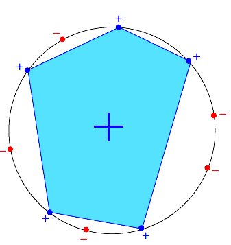
every dichotomy can be implemented by H using a convex region slightly extended from contour of positive inputs。即全部的二分法都可以用于该凸集，中间由正样本连成的蓝色凸区域，便是分割函数 dichotomy 的表现形式，并且可以推导出：

\[m_{\mathcal{H}}(N)=2^{N} \Longleftrightarrow \text{exists } N \text{ inputs that can be shattered} \]

即这种情况叫做可以被shattered。

由上述推导可知存在成长函数为多项式（polynomial）\(m_{\mathcal{H}}(N) = poly(N)\) 可以用于替换原来的\(M\)，但是也存在为指数函数（exponential）的时候这时便不能保证可以替换。

限制函数（bounding function）

在此之前了解一下中断点的概念

中断点（Break Point）：通过观察可以发现，随着训练样本数\(k\)的增加，可能会出现不能够被shatter的现象，第一个不能给shatter的\(k\)记为“minimum break point”，即最小中断点，并且易证得后续\(k+1,k+2,...\)也是中断点。所以当\(N > k\)的时候，该最小中断点会限制 maximum possible \(m_{\mathcal{H}}(N)\)。

限制函数的定义便由中断点而来：

\(B(N; k)\): maximum possible \(m_{\mathcal{H}}(N)\) when break point = \(k\)。即与中断点相对应的成长函数。

并且可以推导出\(B(N, k) \leq B(N-1, k)+B(N-1, k-1)\)。即该限制函数是具有上限的，并且可以最终推导出：

\[B(N, k) \leq \underbrace{\sum_{i=0}^{k-1}\left(\begin{array}{c} N \\ i \end{array}\right)}_{\text {highest term } N^{k-1}} \]

即最高次是\(N^{k-1}\)的多项式即\(poly(N)\)。

Vapnik-Chervonenkis (VC) bound

理想状态下误差关系为：

\[\mathbb{P}\left[\exists h \in \mathcal{H} \text { s.t. }\left|E_{\text {in }}(h)-E_{\text {out }}(h)\right|>\epsilon\right] \leq 2 \quad m_{\mathcal{H}}(N) \cdot \exp \left(-2 \quad \epsilon^{2} N\right) \]

但是真实情况下是经典的 VC bound：

\[\begin{aligned} \mathbb{P}\left[\exists h \in \mathcal{H} \text { s.t. }\left|E_{\text {in }}(h)-E_{\text {out }}(h)\right|>\epsilon\right] & \leq 2 \cdot 2 m_{\mathcal{H}}(2 N) \cdot \exp \left(-2 \cdot \frac{1}{16} \epsilon^{2} N\right) \\ & \leq 4 m_{\mathcal{H}}(2 N) \cdot \exp \left(- \frac{1}{8} \epsilon^{2} N\right) \end{aligned} \]

下面推导 VC bound 是如何获得的！

VC Bound 的获取

第一步：替换\(E_{\text {out}}\)，replace \(E_{\text {out}}\) by \(E_{\text {in}}^{\prime}\)

因为 \(E_{\text {out}}\) 是针对无穷数据求取的，那么便需要使用大小为 \(N\) 的验证数据集 \(\mathcal{D}^{\prime}\) （又叫做 ghost data，因为这只是想象说再抽取一些数据）计算 \(E_{\text {in}}^{\prime}\)。

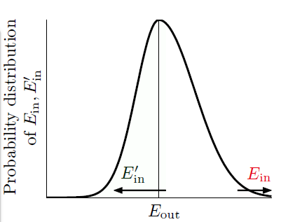
上述分布图，阐释的是如果 \(E_{\text {in}}\) 和 \(E_{\text {out}}\) 相差很远的话，有很大的概率（\(\frac{1}{2}\)）， \(E_{\text {in}}^{\prime}\) 和 \(E_{\text {out}}\) 相差很远。

\[\text{BAD } h \text{ of } E_{\text {in }}-E_{\text {out }} \stackrel{\text { probably }}{\Longrightarrow} \text{BAD } h \text{ of } E_{\text {in }}-E_{\text {in }}^{\prime} \]

可以获得以下不等式（\(\frac{\epsilon}{2}\) 是数学上的放缩，这里未展示具体推导）：

\[\begin{aligned} & \frac{1}{2} \mathbb{P}\left[\exists h \in \mathcal{H} \text { s.t. }\left|E_{\text {in }}(h)-E_{\text {out }}(h)\right|>\epsilon\right] \\ \leq & \mathbb{P}\left[\exists h \in \mathcal{H} \text { s.t. }\left|E_{\text {in }}(h)-E_{\text {in }}^{\prime}(h)\right|>\frac{\epsilon}{2}\right] \end{aligned} \]

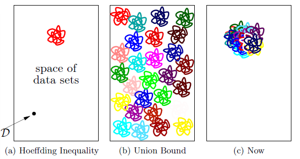
第二步将 \(\mathcal{H}\) 按种类拆解，decompose \(\mathcal{H}\) by kind

因为现在已有的数据大小为\(2N\)，\(\mathcal{H}\) 的最多种类数为\(m_{\mathcal{H}}(2 N)\)。因为 \(E_{\text {in}}\) 和 \(E_{\text {in}}^{\prime}\) 是由 \(\mathcal{D}\) 和 \(\mathcal{D}^{\prime}\) 决定的，那么同类的 hypothesis 其 \(E_{\text {in}}\) 和 \(E_{\text {in}}^{\prime}\) 几乎是相同的，那么便可以使用 union bound 实现由下图中的（b）向（c）的转换。

数学表达为：

\[\begin{aligned} \mathrm{BAD} & \leq 2 \mathbb{P}\left[\exists h \in \mathcal{H} \text { s.t. }\left|E_{\text {in }}(h)-E_{\text {in }}^{\prime}(h)\right|>\frac{\epsilon}{2}\right] \\ & \leq 2 m_{\mathcal{H}}(2 N) \mathbb{P}\left[\text { fixed } h \text { s.t. }\left|E_{\text {in }}(h)-E_{\text {in }}^{\prime}(h)\right|>\frac{\epsilon}{2}\right] \end{aligned} \]

第三步使用无放回海弗丁不等式 ，Use Hoeffding without Replacement

先进行一下变换

\[\left|E_{\mathrm{in}}-E_{\mathrm{in}}^{\prime}\right|>\frac{\epsilon}{2} \Leftrightarrow\left|\frac{E_{\mathrm{in}}}{2}-\frac{E_{\mathrm{in}}^{\prime}}{2}\right|>\frac{\epsilon}{4} \Leftrightarrow\left|E_{\mathrm{in}}-\frac{E_{\mathrm{in}}+E_{\mathrm{in}}^{\prime}}{2}\right|>\frac{\epsilon}{4} \]

那么 \(\frac{E_{\mathrm{in}}+E_{\mathrm{in}}^{\prime}}{2}\) 可以视为由 \(\mathcal{D}\) 和 \(\mathcal{D}^\prime\)组合的数据集的整体的\(E_{\text{in}}\)。那么根据海弗丁不等式可以得出：

\[\mathbb{P}\left[\text { fixed } h \text { s.t. }\left|E_{\text {in }}(h)-\frac{E_{\mathrm{in}}+E_{\mathrm{in}}^{\prime}}{2}\right|>\frac{\epsilon}{4}\right] \leq 2 \exp \left(-2\left(\frac{\epsilon}{4}\right)^{2} N\right) \]

那么 BAD 可以进一步缩放求取上限：

\[\begin{aligned} \mathrm{BAD} & \leq 2 m_{\mathcal{H}}(2 N) \mathbb{P}\left[\text { fixed } h \text { s.t. }\left|E_{\text {in }}(h)-E_{\text {in }}^{\prime}(h)\right|>\frac{\epsilon}{2}\right] \\ & \leq 2 m_{\mathcal{H}}(2 N) \cdot 2 \exp \left(-2\left(\frac{\epsilon}{4}\right)^{2} N\right) \end{aligned} \]

有了VC bound，那么如果满足一下三个条件，那么机器学习便是可行的了！

1. \(m_{\mathcal{H}}(N)\) breaks at \(k\)
2. \(N\) large enough \(\Longrightarrow\) probably generalized \(E_{\text {out }} \approx E_{\text {in }}\)
3. \(\mathcal{A}\) picks a \(g\) with small \(E_{\text {in }} \quad(\text { good } \mathcal{A})\)

VC Dimension

表示符号为 \(d_{vc}\) ，实际上就是可以被 shatter 的最大的输入（训练样本数）。那么可以得出其有以下的性质：

\[\text { if } N \geq 2, d_{\mathrm{vc}} \geq 2, m_{\mathcal{H}}(N) \leq N^{d_{\mathrm{VC}}} \]

那么只需要hypothesis的 \(d_{vc}\) 是有限个的，那么在最坏的情况下，最终获得的 \(g\) 仍然可以保证 \(E_{\text {in}} \approx E_{\text {out}}\)，且与输入的数据分布，学习算法以及目标函数无关。

那么根据该性质将VC bound 重新写为：

For any \(g=\mathcal{A}(\mathcal{D}) \in \mathcal{H}\) and 'statistical' large \(\mathcal{D},\) for \(N \geq 2, d_{\mathrm{vC}} \geq 2\)

\[\mathbb{P}_{\mathcal{D}}[\underbrace{\left|E_{\text {in }}(g)-E_{\text {out }}(g)\right|>\epsilon]}_{\text {BAD }} \leq \underbrace{4(2 N)^{d_{\text {vo }}} \exp \left(-\frac{1}{8} \epsilon^{2} N\right)}_{\delta} \]

那么现在令\(\delta =4(2 N)^{d_{v c}} \exp \left(-\frac{1}{8} \epsilon^{2} N\right)\)，可以推导得：

\[\begin{aligned} \frac{\delta}{4(2 N)^{d_{V C}}} &=\exp \left(-\frac{1}{8} \epsilon^{2} N\right) \\ \ln \left(\frac{4(2 N)^{d_{V C}}}{\delta}\right) &=\frac{1}{8} \epsilon^{2} N \\ \sqrt{\frac{8}{N} \ln \left(\frac{4(2 N)^{d_{V C}}}{\delta}\right)} &=\epsilon \end{aligned} \]

那么\(E_{\text {in}}\)与\(E_{\text {out}}\)的关系可以写为：

\[\begin{aligned} &\text { gen. error }\left|E_{\text {in }}(g)-E_{\text {out }}(g)\right| \quad \leq \quad \underbrace{\sqrt{\frac{8}{N} \ln \left(\frac{4(2 N)^{d_{V}}}{\delta}\right)}}_{\Omega(N, \mathcal{H}, \delta)}\\ &E_{\mathrm{in}}(g)-\sqrt{\frac{8}{N} \ln \left(\frac{4(2 \mathrm{N}) \mathrm{d} \mathrm{v}}{\delta}\right)} \leq E_{\mathrm{out}}(g) \leq E_{\mathrm{in}}(g)+\sqrt{\frac{8}{N} \ln \left(\frac{4(2 N)^{d_{\mathrm{VC}}}}{\delta}\right)} \end{aligned} \]

这里的\(\Omega(N, \mathcal{H}, \delta)\)叫做模型复杂度惩罚项（penalty for model complexity）。

这里给出随着\(d_{vc}\)的变化，三者的变化：

可以看出

• \(d_{\mathrm{vc}} \uparrow: E_{\mathrm{in}} \downarrow\) but \(\Omega \uparrow\)
• \(d_{\mathrm{vc}} \downarrow: \Omega \downarrow\) but \(E_{\mathrm{in}} \uparrow\)
• best \(d_{\mathrm{vc}}^{*}\) in the middle

所以说并不是hypothesis越强（越强复杂度越高，惩罚项越大）越好，适中才是最好的状态。

理论推导需要 \(N \approx 10,000 d_{v c}\) 大小的数据，实践过程中发现可能只需要 \(N \approx 10 d_{v c}\) 大小的数据，因为在求取VC bound的过程中使用了太多的缩放。因为其适用于任何分布（distribution），任何目标函数（target function），任何数据（data），任何模型（hypothesis）以及任何选择学习算法（algorithm）。所以说 VC bound 的物理意义对于提高机器学习算法是很重要的。

已有数据误差最小 \(E_{\text {in}} \approx 0\)

训练数据误差最小需要通过学习算法选取假设函数实现，在前边的PLA中证明了，最终可以获取到 \(\mathbf{w}_t = \mathbf{w}_f\)，即 \(E_{\text {in}} \approx 0\)

那么根据 \(E_{\text {in}} \approx E_{\text {out}}, E_{\text {in}} \approx 0\) 可以得出 \(E_{\text {out}} \approx 0\)。也就是说如果有充足的数据（large \(N\)），好的 hypothesis (finite \(d_{\mathrm{vc}}\)) 和 algorithm (low \(E_{in}\)) 可以保证 \(E_{\text {out}} \approx 0\)，即机器学习算法是可行的。

噪声（Noise）

噪声的表现形式就是 当 \(\mathbf{x} \sim P(\mathbf{x})\) 时 \(y \sim P(y | \mathbf{x})\)，即\(y\)并非一个固定值，而是符合某种分布的变量。事实证明（不在推导），VC bound 仍然适用，即：

\[\text { VC holds for } \underbrace{\mathbf{x}^{i, i, d} \cdot P(\mathbf{x}), y^{i, i, d} \cdot P(y | \mathbf{x})}_{(\mathbf{x}, y)^{i, i, d} \cdot P(\mathbf{x}, y)} \]

那么学习目标变为：利用已有的常见输入 (w.r.t. \(P(\mathbf{x}))\) 预测 ideal mini-target (w.r.t. \(P(y | \mathbf{x}))\) （\(y\)的分布函数）

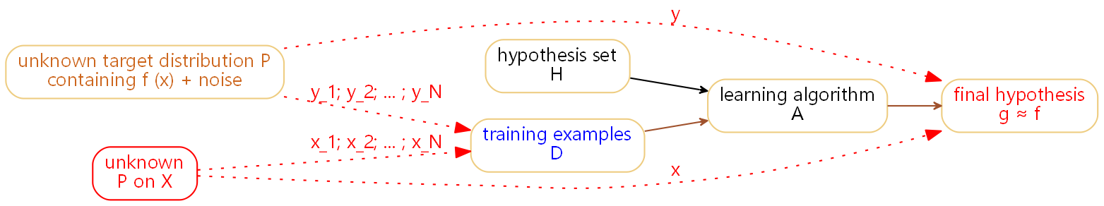
那么掺杂噪声之后的机器学习流程图改变如下：

误差测量（Error Measure)

之前使用的测量方法是 0/1 误差( 0/1 error )：

\[E_{\text {out }}(g)=\underset{\mathbf{x} \sim P}{\mathcal{E}}\underbrace{[\kern-0.15em[g(\mathbf{x}) \neq f(\mathbf{x})]\kern-0.15em]}_{err(g(x),f(x))} \]

其中 \(err\) 是每个点的误差测量方法（pointwise error measure）。那么 \(E_{\text {in}}\) 和 \(E_{\text {out}}\) 可以写为：

\[E_{\mathrm{in}}(g)=\frac{1}{N} \sum_{n=1}^{N} \operatorname{err}\left(g\left(\mathbf{x}_{n}\right), f\left(\mathbf{x}_{n}\right)\right) \quad E_{\mathrm{out}}(g)=\underset{x \sim p}{\mathcal{E}} \operatorname{err}(g(\mathbf{x}), f(\mathbf{x})) \]

还有一种经典的误差测量方法：方差（squared error）

\[\operatorname{err}(\tilde{y}, y)=(\tilde{y}-y)^{2} \]

加权分类（Weighted Classification）

也就是说当分类结果错误时的惩罚大小不同，这里列举二分类时，权重分别为：\(1,\text{w}_{negative}\)

\[E _ { \text{in} } ^ { \text{w} } ( h ) = \frac { 1 } { N } \sum _ { n = 1 } ^ { N } \left\{ \begin{array} { c l } { 1 } & { \text { if } y _ { n } = + 1 } \\ { \text{w}_{negative} } & { \text { if } y _ { n } = - 1 } \end{array} \right\} \cdot [ y _ { n } \neq h ( x _ { n } ) ] \]

一般的想法：

PLA: 无所谓，只要是线性可分的即可。
pocket: 修改 pocket-replacement rule（替换策略），即如果 \(\text{w}_{t+1}\) 对应的 \(E _ { \text{in} } ^ { \text{w} }\) 比 \(\hat{\text{w}}\) 更小，用 \(\text{w}_{t+1}\) 替换 \(\hat{\text{w}}\) 。

当然除了加大系数，还可以使用 ‘virtual copying’ ：

• weighted PLA： 随机检测负样本错误 \(\text{w}_{negative}\) 次
• weighted pocket replacement（替换策略）：如果 \(\text{w}_{t+1}\) 对应的 \(E _ { \text{in} } ^ { \text{w} }\) 比 \(\hat{\text{w}}\) 更小，用 \(\text{w}_{t+1}\) 替换 \(\hat{\text{w}}\) 。

如果使用拷贝会导致数据不平衡，那么改变惩罚系数可能更合适。