机器学习week2 ex1 review

这周的作业主要关于线性回归。

1. Linear regression with one variable

1.1 Plotting the Data

通过已有的城市人口和盈利的数据，来预测在一个新城市营业的收入。
文件ex1data1.txt包含了以下数据：

第一列是城市人口数据，第二列是盈利金额（负数代表亏损）。
可以首先通过绘图来直观感受。
这里我们可以使用散点图（scatter plot ）。
通过 Octave/MATLAB 实现。
数据存储在ex1data1.txt中，如下图所示：

文件ex1.m将ex1data1.txt中的所有数据载入data：
```
data = load('ex1data1.txt');      % read comma separated data
```

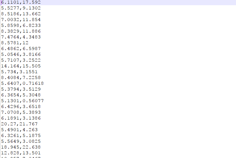
Octave/MATLAB 会根据数据文件中的逗号来分隔数据。这里的data以矩阵形式存储。因为有两组数据，所以是两列。
然后分别将人口和盈利存入 $X$ 和 $y$ 中。

X = data(:,1); y = data(:,2);
m = length(y);

$X$ 取data的第一列， $y$ 取第二列。 $m$ 是 training example 的数量。因为 $X$ 和 $y$ 大小相同，用哪个都无所谓。

下一步调用 PlotData 函数绘制散点图。
我们需要首先把这个函数补充完整。
这是文件中包含的原始版本：

function plotData
%PLOTDATA Plots the data points x and y into a new figure 
%   PLOTDATA(x,y) plots the data points and gives the figure axes labels of
%   population and profit.

figure; % open a new figure window

% ====================== YOUR CODE HERE ======================
% Instructions: Plot the training data into a figure using the 
%               "figure" and "plot" commands. Set the axes labels using
%               the "xlabel" and "ylabel" commands. Assume the 
%               population and revenue data have been passed in
%               as the x and y arguments of this function.
%
% Hint: You can use the 'rx' option with plot to have the markers
%       appear as red crosses. Furthermore, you can make the
%       markers larger by using plot(..., 'rx', 'MarkerSize', 10);





% ============================================================

end

我们可以看到他要求我们绘制散点图，并给横纵坐标加上 population 和 profit 的标签。
Hint 提示我们这样做：

使用figure打开一个图形窗口。

使用plot函数绘图。用xlabel和ylabel分别设置横纵坐标的标签。rx将散点设置为红十字形（red cross）。通过'Markersize'，10'设置散点大小。

代码如下：

plot(x, y, 'rx', 'Markersize', 10);           % plot the data
ylabel('Profit in $10,000s');                 % set the y-axis label
xlabel('Population of City in 10,000s');      % set the x-axis label

这时再运行ex1.m,就可以得到如下图形：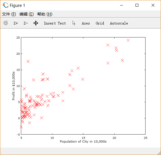
Figure 1: Scatter plot of training data

1.2 Gradient Descent

通过梯度下降算法计算线性回归参数 $\theta$ 。

1.2.1 Update Equations

线性回归的目标就是使代价函数最小
$J(\theta) = \displaystyle{\frac {1} {2m}\sum_{i=1}^{m}}(h_\theta(x^{(i)})-y^{(i)})^2$
其中
$h_\theta(x) = \theta^Tx = \theta_0+\theta_1x_1$

使用批量梯度下降法（batch gradient descent ) 以使 $J(\theta)$ 最小。
$\theta_j := \theta_j -\alpha \displaystyle{\frac{1}{m}\sum_{i=1}^{m}}(h_\theta(x^{(i)})-y^{(i)})x_j^{(i)}$
( simultaneously update $\theta_j$ for all $j$ )

1.2.2 Implementation

目前的 $X$ 是一个列向量，每一行存储一个 training example，即 $x_1$ 。
因此在脚本文件ex1.m中，为了处理 $\theta_0$ , 给每一行增加一个 $x_0 = 1$ 。

X = [ones(m,1) data(:,1)];   % Add a column of ones to x

因为只有一个变量 $x_1$ 影响盈利，
$\theta = \left[ \begin{matrix} \theta _{0}\\\theta _{1}\end{matrix} \right]$
初始化 $\theta$ 为 $\left[ \begin{matrix} 0 \\ 0 \end{matrix} \right]$

theta = zeros(2,1);  % initialize fitting parameters

设置迭代次数和 $\alpha$ 的值：

iterations = 1500;
alpha = 0.01;

1.2.3 Computing the cost $J(\theta)$

根据上述公式，完成computeCost以计算代价函数 $J(\theta)$

function J = computeCost(X, y, theta)
%COMPUTECOST Compute cost for linear regression
%   J = COMPUTECOST(X, y, theta) computes the cost of using theta as the
%   parameter for linear regression to fit the data points in X and y

% Initialize some useful values
m = length(y); % number of training examples
prediction = X * theta;
sqError = (prediction - y).^2;

% You need to return the following variables correctly 
J = 0;

% ====================== YOUR CODE HERE ======================
% Instructions: Compute the cost of a particular choice of theta
%               You should set J to the cost.

J = 1/(2 * m) * sum(sqError);



% =========================================================================

end

我们来看一下脚本文件ex1.m中这一部分的测试代码

fprintf('\nTesting the cost function ...\n')
% compute and display initial cost
J = computeCost(X, y, theta);
fprintf('With theta = [0 ; 0]\nCost computed = %f\n', J);
fprintf('Expected cost value (approx) 32.07\n');

% further testing of the cost function
J = computeCost(X, y, [-1 ; 2]);
fprintf('\nWith theta = [-1 ; 2]\nCost computed = %f\n', J);
fprintf('Expected cost value (approx) 54.24\n');

fprintf('Program paused. Press enter to continue.\n');
pause;

它对两组数据进行了测试。一组是我们之前初始化后的 $\theta = \left[ \begin{matrix} 0 \\ 0 \end{matrix} \right]$ , 另一组是 $\left[ \begin{matrix} -1 \\ 2 \end{matrix} \right]$ 。
如果你的computeCost.m计算正确的话，输出的两个答案应该是32.072734和54.242455。

1.2.4 Gradient descent

根据之前的公式
$\theta_j := \theta_j -\alpha \displaystyle{\frac{1}{m}\sum_{i=1}^{m}}(h_\theta(x^{(i)})-y^{(i)})x_j^{(i)}$
( simultaneously update $\theta_j$ for all $j$ )

补充gradientDescent.m的代码。如下：

%GRADIENTDESCENT Performs gradient descent to learn theta
%   theta = GRADIENTDESCENT(X, y, theta, alpha, num_iters) updates theta by 
%   taking num_iters gradient steps with learning rate alpha

% Initialize some useful values
m = length(y); % number of training examples
J_history = zeros(num_iters, 1);
temp = theta;
n = length(theta);

for iter = 1:num_iters

    % ====================== YOUR CODE HERE ======================
    % Instructions: Perform a single gradient step on the parameter vector
    %               theta. 
    %
    % Hint: While debugging, it can be useful to print out the values
    %       of the cost function (computeCost) and gradient here.
    %
    for j = 1:n
        temp(j) = theta(j) - 1/m*alpha*sum((X*theta-y).*X(:,j));
    end;
    theta = temp;






    % ============================================================

    % Save the cost J in every iteration    
    J_history(iter) = computeCost(X, y, theta);

end

end

事实上这已经解决了多变量的线性回归问题，尽管这里只用处理 $n=2$ 的情况。

再来看一下脚本文件里这一部分的内容：

fprintf('\nRunning Gradient Descent ...\n')
% run gradient descent
theta = gradientDescent(X, y, theta, alpha, iterations);

% print theta to screen
fprintf('Theta found by gradient descent:\n');
fprintf('%f\n', theta);
fprintf('Expected theta values (approx)\n');
fprintf(' -3.6303\n  1.1664\n\n');

% Plot the linear fit
hold on; % keep previous plot visible
plot(X(:,2), X*theta, '-')
legend('Training data', 'Linear regression')
hold off  % do not overlay any more plots on this figure

% Predict values for population sizes of 35,000 and 70,000
predict1 = [1, 3.5] *theta;
fprintf('For population = 35,000, we predict a profit of %f\n',...
    predict1*10000);
predict2 = [1, 7] * theta;
fprintf('For population = 70,000, we predict a profit of %f\n',...
    predict2*10000);

fprintf('Program paused. Press enter to continue.\n');
pause;

使用梯度下降法后输出计算得到的 $\theta$ :
image_1btongdv2afu1dae13bv1e3i1mimm.png-7.7kB
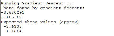
与正确情况吻合。

之后绘制图线。对之前的散点图使用hold on，保留图形。
再绘制经过梯度下降后得到的 $X$ 和 $h_\theta(x) = X\theta$ 的图线。
得到如下图形：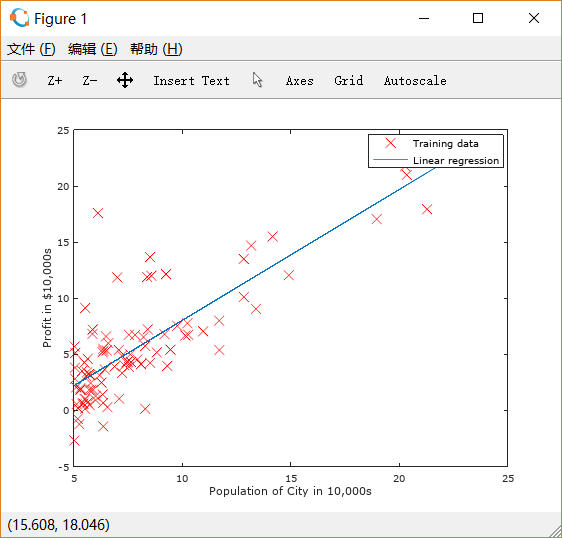
image_1bton9ngt29919hc1duq3uh9339.png-36kB
再对population = 35000 和 70000的情况进行估计，输出这两种情况下的估计值：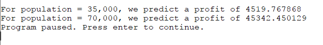
image_1btoni94o1rg9d14107ktcu1oat13.png-8.5kB

1.3 Visualizing $J(\theta)$

脚本文件ex1.m提供了对 $J(\theta)$ 可视化的部分。

fprintf('Visualizing J(theta_0, theta_1) ...\n')

% Grid over which we will calculate J
theta0_vals = linspace(-10, 10, 100);
theta1_vals = linspace(-1, 4, 100);

函数 linspace（BASE,LIMIT,N=100) 返回一个从BASE到LIMIT的等间距分布的行向量；如果BASE和LIMIT是列向量的话，返回一个矩阵。不输入N的时候默认为100。

% initialize J_vals to a matrix of 0 s
J_vals = zeros(length(theta0_vals), length(theta1_vals));

% Fill out J_vals
for i = 1:length(theta0_vals)
    for j = 1:length(theta1_vals)
      t = [theta0_vals(i); theta1_vals(j)];
      J_vals(i,j) = computeCost(X, y, t);
    end
end

对 $\theta_0$ 和 $\theta_1$ 平面上的点求出其代价函数值。
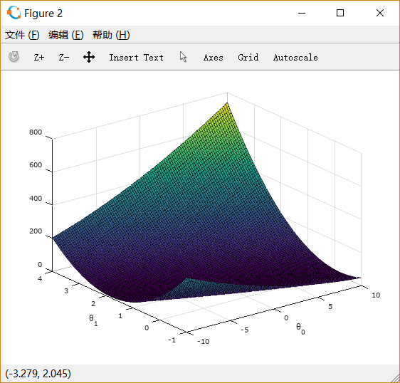
绘制曲面图：

% Because of the way meshgrids work in the surf command, we need to
% transpose J_vals before calling surf, or else the axes will be flipped
J_vals = J_vals';
% Surface plot
figure;
surf(theta0_vals, theta1_vals, J_vals)
xlabel('\theta_0'); ylabel('\theta_1');

image_1btorckqkshi1l161shbka43263a.png-179.6kB
绘制等值线图：

% Contour plot
figure;
% Plot J_vals as 15 contours spaced logarithmically between 0.01 and 100
contour(theta0_vals, theta1_vals, J_vals, logspace(-2, 3, 20))
xlabel('\theta_0'); ylabel('\theta_1');
hold on;
plot(theta(1), theta(2), 'rx', 'MarkerSize', 10, 'LineWidth', 2);

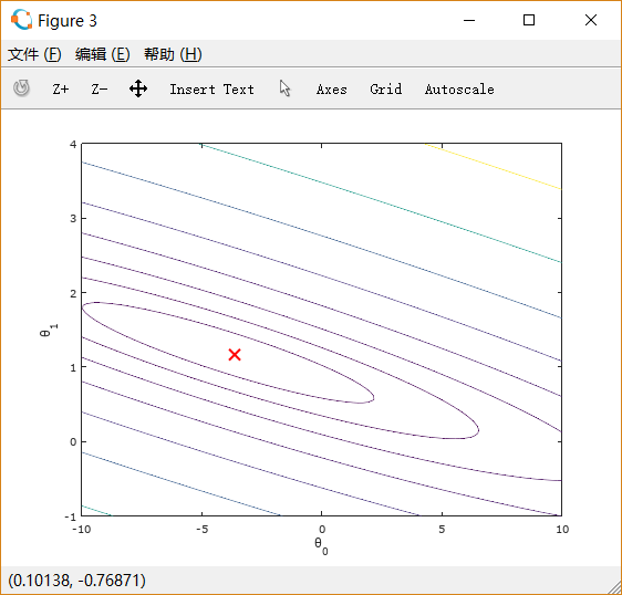
image_1btordvej9j1e3sdun1lvcnm33t.png-53.8kB
从图中可以看出最小值所在的位置。

2. Linear regression with multiple variables

这一次需要处理多变量的线性回归。比如预测房价，需要考虑的因素可能就包括房子的大小、卧室的数量。
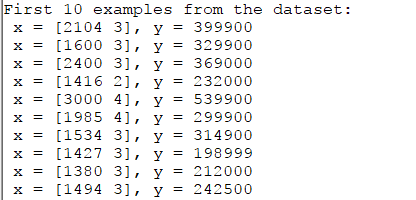
在文件ex1data2.txt中有多变量的 training example。如下图所示：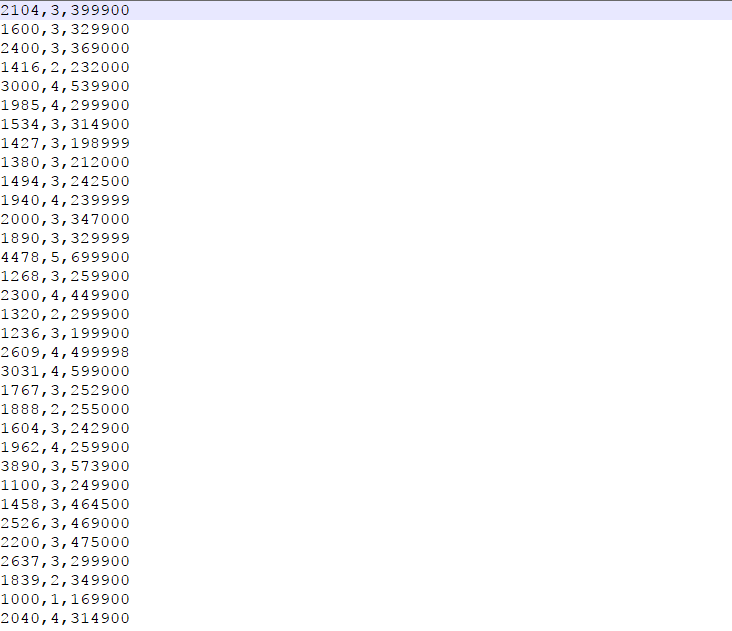
image_1btorn0cm5f9vrqa3i1tjr1n374a.png-40.5kB
共有三列，第一列是房子面积（单位：平方英尺），第二列是卧室数量，第三列是房价。

2.1 Feature normalization

脚本文件ex1_multi中首先展示部分数据：

%% Load Data 
data = load('ex1data2.txt');
X = data(:, 1:2);
y = data(:, 3);
m = length(y);

% Print out some data points
fprintf('First 10 examples from the dataset: \n');
fprintf(' x = [%.0f %.0f], y = %.0f \n', [X(1:10,:) y(1:10,:)]');

fprintf('Program paused. Press enter to continue.\n');
pause;

image_1btos2cq66mm8d91d00oa21v14n.png-12.3kB
通过观察数据可以发现，第一列数据大小比第二列数据高三个数量级，需要进行标准化（Normalization ）
标准化包括如下步骤：

减去平均值
除以标准差（因为大部分数据会落在平均值 $\pm$ 标准差的范围内），也可以直接选择用max-min来代替

代码如下：

function [X_norm, mu, sigma] = featureNormalize(X)
%FEATURENORMALIZE Normalizes the features in X 
%   FEATURENORMALIZE(X) returns a normalized version of X where
%   the mean value of each feature is 0 and the standard deviation
%   is 1. This is often a good preprocessing step to do when
%   working with learning algorithms.

% You need to set these values correctly
X_norm = X;
mu = zeros(1, size(X, 2));
sigma = zeros(1, size(X, 2));

% ====================== YOUR CODE HERE ======================
% Instructions: First, for each feature dimension, compute the mean
%               of the feature and subtract it from the dataset,
%               storing the mean value in mu. Next, compute the 
%               standard deviation of each feature and divide
%               each feature by it's standard deviation, storing
%               the standard deviation in sigma. 
%
%               Note that X is a matrix where each column is a 
%               feature and each row is an example. You need 
%               to perform the normalization separately for 
%               each feature. 
%
% Hint: You might find the 'mean' and 'std' functions useful.
% 

mu = mean(X);
sigma = std(X);
for i = 1:size(X,1)
   X_norm(i,:) = (X(i,:)-mu)./sigma;
end;









% ============================================================

end

mean 和 std 分别用来计算向量的平均值和标准差，如果是对象是矩阵的话，默认计算每列的平均值和标准差，然后返回一个行向量。

2.2 Gradient descent

这一部分（包括梯度下降和代价函数），我们在单变量的时候处理的时候已经可以用于多变量了。略去。
值得一提的是，在计算代价函数的时候，用如下方法计算是很有效的：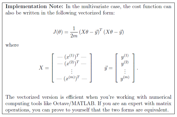
image_1btot5mnqv7tmgp1tce1dhr1cn754.png-56.1kB

2.2.1 Selecting learning rates

可以通过修改ex1_multi.m中的learning rate来直观感受其作用。
其中有如下代码：

% Init Theta and Run Gradient Descent 
theta = zeros(3, 1);
[theta, J_history] = gradientDescentMulti(X, y, theta, alpha, num_iters);

% Plot the convergence graph
figure;
plot(1:numel(J_history), J_history, '-b', 'LineWidth', 2);
xlabel('Number of iterations');
ylabel('Cost J');

% Display gradient descent's result
fprintf('Theta computed from gradient descent: \n');
fprintf(' %f \n', theta);
fprintf('\n');

这段代码的功能是画出 $J(\theta)$ 随迭代次数的变化情况。
numel函数返回对象的元素个数。
J_history内存储了每次迭代后的代价函数值。在gradientDescentMulti.m中，我们每一次循环中有这样的步骤来计算J_history：

    % Save the cost J in every iteration    
    J_history(iter) = computeCostMulti(X, y, theta);

设置learning rate $\alpha$ 为 0.01，0.03，0.1，1，1.5 画出的图像依次如下所示：

image_1btp4lfg21t7j7fpej21qiq19985h.png-25.4kB
image_1btp4ncpa1cfg1248kei1eec1d195u.png-27.2kB
image_1btp4prvh161v7o9f1e1flsral7b.png-25.3kB
image_1btp4r2nk11181hmjh85f6p13hq7o.png-22kB
image_1btp4vmu3p6rhbi7lrqbkllq85.png-22.4kB
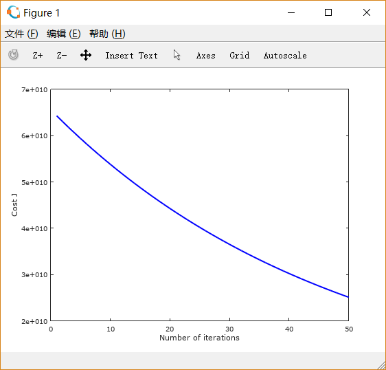
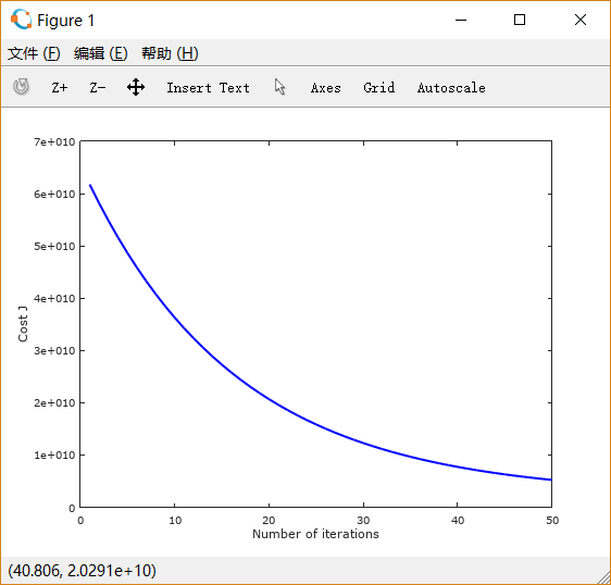
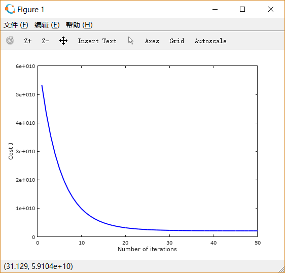
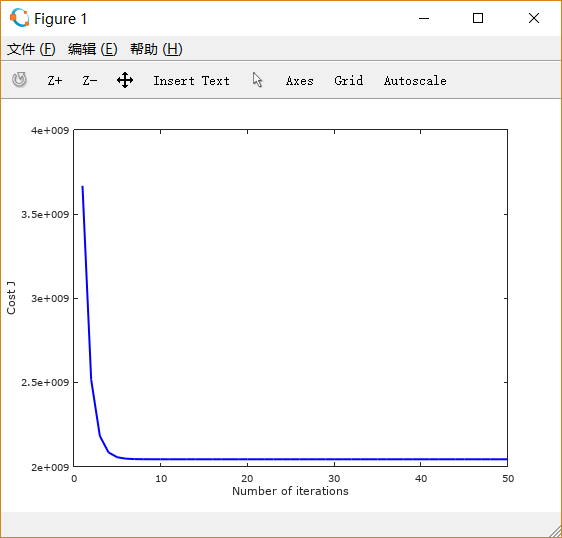
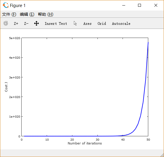
可以注意到，起初 $\alpha$ 设置得很小的时候，下降非常缓慢； $\alpha$ 适当增大之后，下降速度变快；而 $\alpha$ 过大时，图线不降反升。

用梯度下降法在ex1_multi中计算1650平方英尺，3间卧室的房子的价格：

testify = [1,1650, 3];
price = (testify - [0 mu]) ./ [1 sigma] * theta;

需要记得，在使用时要先进行normalization。
输出的结果是：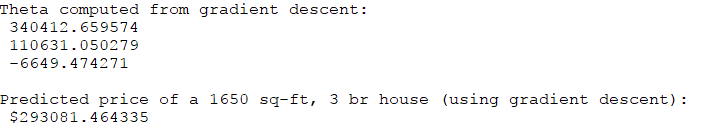
image_1btp6hacsggttin1uvvq4d1io92.png-10.8kB

2.3 Normal equations

$\theta = (X^TX)^{-1}X^T\vec {y}$

代码相当简单：

function [theta] = normalEqn(X, y)
%NORMALEQN Computes the closed-form solution to linear regression 
%   NORMALEQN(X,y) computes the closed-form solution to linear 
%   regression using the normal equations.

theta = zeros(size(X, 2), 1);

% ====================== YOUR CODE HERE ======================
% Instructions: Complete the code to compute the closed form solution
%               to linear regression and put the result in theta.
%

% ---------------------- Sample Solution ----------------------


theta = pinv(X' * X) * X' * y;

% -------------------------------------------------------------

% ============================================================

end

用normal Equation在ex1_multi中计算1650平方英尺，3间卧室的房子的价格：

price = testify * theta;

normal equation 不需要进行normalization。
输出的结果是：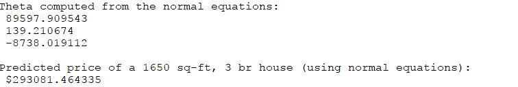
image_1btp6hv3r1uecu3s1sg1osjfdu9f.png-11.1kB

与之前用梯度下降法求出的结果吻合得相当精确。

posted @ 2017-11-01 11:20 EtoDemerzel 阅读(627) 评论(2) 编辑收藏举报

会员力量，点亮园子希望

刷新页面返回顶部

EtoDemerzel

learn to code

机器学习week2 ex1 review

机器学习week2 ex1 review

1. Linear regression with one variable

1.1 Plotting the Data

1.2 Gradient Descent

1.2.1 Update Equations

1.2.2 Implementation

1.2.3 Computing the cost $J(\theta)$

1.2.4 Gradient descent

1.3 Visualizing $J(\theta)$

2. Linear regression with multiple variables

2.1 Feature normalization

2.2 Gradient descent

2.2.1 Selecting learning rates

2.3 Normal equations

公告