[论文阅读 ] Domain generalization via feature variation decorrelation

Domain generalization via feature variation decorrelation

3 METHOD

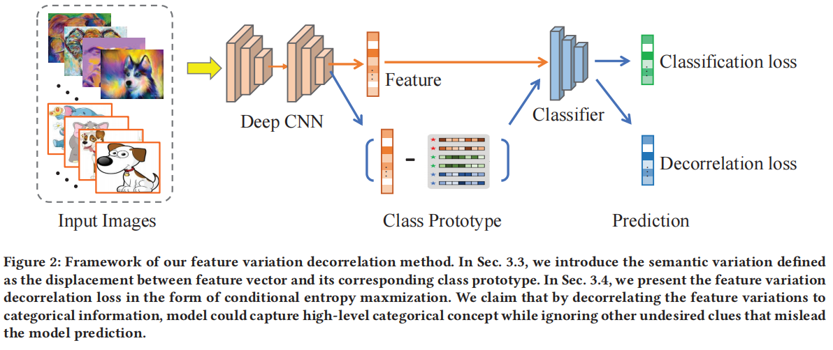
在本节中，我们首先在第3.2节解释我们的动机。然后，在第3.3节中，我们介绍特征变化的解缠和讨论方差转移的想法。最后，在第3.4节中，我们提出了我们的新颖特征变化解相关损失。图2显示了所提出方法的框架。

3.1 Problem Setting

让\(\mathcal{X}\)和\(Y\)分别表示数据和标签空间。在领域泛化（DG）中，有\(K\)个源域\(\left\{\mathcal{D}_i\right\}_{i=1}^K\)和\(L\)个目标域\(\left\{\mathcal{D}_i\right\}_{i=K+1}^{K+L}\)。具体来说，源域数据集表示为\(\mathcal{D}_i=\left\{\left.\left(x_j^i, y_j^i\right)\right|_{j=1} ^{N_i}\right\}\)，其中\(x_j^i\)和\(y_j^i\)分别表示来自第\(i^{th}\)域的第\(j^{\text {th }}\)训练样本及其标签，\(N_i\)是域\(i\)中源图像的数量。需要注意的是，所有域共享相同的标签空间\(\mathcal{Y}\)。DG的目标是将模型在源域样本上的训练推广到未见过的目标域。我们定义一个由\(\theta\)参数化的特征提取器为\(F_\theta\)，由\(\phi\)参数化的分类器为\(C_\phi\)，使得网络可以表示为\(G_{\theta, \phi}(\cdot)=C_\phi \circ F_\theta(\cdot)\)。

3.2 Motivation

我们的方法受到一个观察的启发，即与类别无关的信息，比如样本变化（例如几何变形、背景改变、简单噪音）和域变化（图像风格变化），有时会作为类别预测的线索，导致负迁移[29]，特别是当目标域非常异质化的时候。因此，我们的目标是提出一种方法，通过将语义/域变化与类别信息解耦，从而捕获源域之间的不变性，使得模型在给定未见目标样本时只关注高层次的语义结构进行预测。

由于深度神经网络擅长将输入样本的特征线性化\([34,38]\)，样本之间的语义关系可以通过它们深层特征的空间位置来捕获。我们建议通过减去在线估计的类原型的特征向量，线性解缠特征空间中的观察到的变化。然后，我们使用我们的新损失函数将解缠的变化与类信息进行解耦。通过这样做，我们的模型不会因为基于不想要的变化线索而做出错误的预测而受到影响。

3.3 Variation Disentanglement

在这一部分中，我们首先建立一个特征存储库，根据存储库计算类原型，最终获得语义变化的解缠。

3.3.1 Multi-variate Normal Distribution Assumption.

我们假设数据分布遵循多变量正态分布 \(\mathcal{N}\left(\mu_c, \Sigma_c\right)\)，其中 \(\mu_c\) 和 \(\Sigma_c\) 分别表示类别条件均值向量和协方差矩阵。在接下来的几节中，我们将估计类别条件均值作为类原型，并获取特征的变化。

3.3.2 Online Memory Bank Update.

首先，我们启动模型训练进行几个 epoch，以确保获得有意义的特征空间。然后，我们通过模型提取所有源特征 \(z_j^i=F_\theta\left(x_j^i\right)\) 并将它们保存到特征内存库 \(M=\left\{\left.\left(z_j^i, y_j, d_j\right)\right|_{i=1} ^N\right\}\) 中，其中 \(y_j\) 表示类别标签，\(d_j\) 表示特征 \(z_j^i\) 的域标签。

需要注意的是，我们的内存库 \(M\) 在运行时通过最新的特征进行更新以替换旧的特征。形式上，在每次迭代 k 中，我们将更新内存模块 M 中的一批特征：

\[z_j^M \leftarrow z_j^i, \quad j \in \mathcal{B}^k \tag{1} \]

除了用新特征准确替换旧特征外，我们还考虑以移动平均的方式更新特征。具体来说，内存模块 \(\mathrm{M}\) 中的特征将通过新特征和上一轮旧特征的移动平均进行更新：

\[z_j^t=\gamma z_j+(1-\gamma) z_j^{t-1}, \quad j \in \mathcal{B}^k, \tag{2} \]

其中 \(\gamma\) 是移动平均系数。
更新规则会影响存储在内存库中的特征质量，因此直接关系到语义变化解缠的质量。我们在表格 5 中进行了更新策略的消融研究，并发现方程（1）的性能更好。

3.3.3 Prototype Selection.

我们通过对同一类别的特征取平均来估计类原型。具体而言，类原型 \(y\) 可以表示为：

\[\hat{\mu}_y=\frac{1}{K} \sum_{d=1}^K \hat{\mu}_y^d, \quad \hat{\mu}_y^d=\frac{1}{N_y^d} \sum_{j=1}^{N_y^d} z_j^i, \tag{3} \]

其中 \(K\) 是源域的数量。\(\hat{\mu}_y^d\) 是特定域的类原型。\(N_y^d\) 是类别 \(y\) 和域 \(d\) 中的样本数量。通常，类原型的表示反映了每个类别的神经语义。例如，人脸类别的类原型通常是正面的、具有神经表情的。这激发了我们通过简单地将特征减去其对应的类原型来获取语义特征变化。

3.3.4 Semantic Feature Variation.

我们考虑在潜在特征空间中捕获给定样本的语义信息的变化。形式上，我们将语义变化 \(v_j\) 定义为第 \(\mathrm{j}\) 个特征向量 \(z_j\) 与该特征空间中类别 \(y_j\) 的估计原型之间的偏移量：

\[v_j=z_j-\hat{\mu}_{y_j} \tag{4} \]

这些变化可以代表语义含义，比如形状、颜色、视觉角度和背景等。由于我们为同一类别但不同域的样本使用统一的类原型，因此语义变化 \(v_j\) 也捕获了域变化。我们认为这些变化不应对分类预测产生影响，并在下一节引入一个新的损失函数来削弱这种相关性。

Discussion on variation transfer.

受长尾识别的启发[22]，将方差从头部类别转移到尾部类别，使得尾部类别的样本可以增强，我们也考虑通过类别和域之间的方差转移来增强我们的训练样本。我们不是在原始空间进行操作，而是在特征空间中增强样本。具体来说，我们采用条件 GAN [25] 来生成带有来自其他类别的变化的类别 \(y\) 的新特征。类原型 \(\hat{\mu}_y\) 和变化 \(v_j\) 是生成器 \(G\) 的输入，生成新的带有类别标签 \(y\) 的增强特征 \(z_{\text {aug }}^j\)：

\[z_{\text {aug }}^j=G\left(\hat{\mu}_y, v_j\right) . \tag{5} \]

此外，引入了鉴别器 \(D\) 来区分真实特征和虚假（生成的）特征。鉴别器被优化以最小化以下目标函数，而生成器被优化以最大化它以愚弄鉴别器。

\[\mathcal{L}_{a d v}(G, D)=\frac{1}{N} \sum_{j=1}^N \log D\left(z^j, y_j\right)+\frac{1}{N} \sum_{j=1}^N \log D\left(1-G\left(\hat{\mu}_y, v_j\right), y\right), \tag{6} \]

其中 \(N\) 是所有源样本的数量。
我们将这些增强的特征纳入训练，并在表 5 中报告了通过特征增强进行的方差转移的结果。我们发现与基本模型相比，这种方法取得了轻微的改善。请查看 4.5.1 节以了解更多详细信息。

3.4 Feature Variation Decorrelation

我们方法的关键思想是，真实数据的观察变化（如几何变形、背景变化、简单噪声和域风格）不应影响模型的分类预测，从而使模型只关注于高层次的分类概念进行学习，并更好地推广到未见过的领域。

首先，我们在来自源域样本的基础上训练我们的模型，采用以下目标：

\[\min _{\mathcal{F}, C} \frac{1}{N} \sum_{j=1}^N \mathcal{L}_{c e}\left(C\left(\mathcal{F}\left(x_j\right)\right), y_j\right), \tag{7} \]

其中 \(\mathcal{L}_{c e}\) 表示交叉熵损失。

为了解相关分类信息和变化之间的关系，我们提出了一种新颖的特征变化解相关（FVD）损失，通过使特征变化的分类器预测具有均匀分布的特性来推动。具体而言，我们根据方程 4 计算特征的变化，将其输入分类器，并最大化这种预测的条件熵。变化预测的条件熵可以形式化地表示为：

\[\mathcal{L}_{F V D}=-\frac{1}{N} \sum_{j=1}^N C\left(\mathcal{F}\left(x_j\right)-\mu_{y_j}\right) \log \left(C\left(\mathcal{F}\left(x_j\right)-\mu_{y_j}\right)\right) . \tag{8} \]

通过最大化 \(\mathcal{L}_{F V D}\)，变化的分类器预测将接近于均匀分布的向量。换句话说，它与分类信息没有任何相关性。

最后，总损失函数可以表示为：

\[\mathcal{L}_{\text {all }}=\mathcal{L}_{c e}-\lambda \mathcal{L}_{F V D}, \tag{9} \]

其中 \(\lambda\) 是平衡解相关损失的超参数。

4.5 Ablation Study

4.5.1 Feature Variation Decorrelation vs Feature Augmentation.

As discussed in Section 3.3.4, semantic feature variation could be utilized to augment the features of one class along the direction of unseen variations from other class. This is based on the motivation that humans are capable of transferring variations from one visual class to another or from one domain to another. For example, when we see an animal that we have never seen before, we can imagine how it will look with different background and surroundings. As Table 5 reports, feature augmentation achieves a marginal improvement compared to the vanilla baseline by 1.51%. In comparison, feature variation decorrelation largely outperform feature augmentation by 4.61%. The possible reason of limited improvement from feature augmentation is that the generated features are still within the similar mode of original data distribution. In comparison, variation decorrelation can be considered as an implicit way to achieve inter-class variance transfer by regularizing the feature variations to be class-agnostic. Therefore, the sample variations could be implicitly shared across classes.

4.5.2 Feature Variation Decorrelation vs Feature Disentanglement.

Our method also shares some similarity with representation disentanglement such as DADA [29] where a feature is disentangled into domain-invariant, domain-specific and class-irrelevant features. Different from our method, DADA disentangles the feature with additional disentangler network and uses auto-encoder to reconstruct the original feature. During the training and testing, only domain-invariant feature is used for class prediction in DADA while our method uses original feature for model prediction. In comparison, our method does not specially disentangle the feature into several components but regularizing the variation portion of original feature to be class-agnostic. We implemented DADA in Table 5 and term it as DisETG. It is reported that our feature correlation achieves a large margin over DADA by 4.75%, which demonstrates the effectiveness of our method over representation disentanglement method.

4.5.3 Importance of Memory Bank Updating Rule.

As Section 3.3.2 presents, we introduce two online updating rule for memory bank: One is to replace the old features with current new features, the other is to replace the old ones with the moving average of current features. We term the former option as "New" and the latter as "Moving Avg" in Table 5. It is reported that using "New" as memory bank updating rule achieves the better performance than using "Moving Avg" by 1.27% for decorrelation experiment and by 0.69 % for feature augmentation experiment. The reason might be that the moving average of feature accumulate the out-of-date features and bias the estimation of class prototype.

4.5.4 Hyper-parameter Sensitivity .

We conduct hyperparaemter sensitivity experiment on from Equation 9 and report the result in figure 5. We choose from {0, 0.1, 0.5, 1, 2} for sensitivity experiment. The findings can be summarized as follows: (1) When is larger than zero (which means our feature variation decorrelation loss is applied), our model has been improved drastically compared to the vanilla baseline. (2) The model achieves the best performance with 85.44% when is equal to 0.1. (3) Our model is robust to the changes of hyper-parameter between {0.1, 0.5, 1, 2}.

4.6 Qualitative Analysis

4.6.1 Feature Visualization.

To better understand the distribution of the learned features, we exploit t-SNE [23] to analyze the feature space learned by vanilla baseline and our feature decorrelation on PACS dataset with art painting as target domain in figure 3 (a) and (b). We can qualitatively observe that our method could learn more discriminative feature space where clusters are more compact and domain-invariant than vanilla baseline.

4.6.2 Visualization of Prototype.

To validate our prototype computed based on recorded memory feature bank could capture the high-level categorical information, we use the domain-specific prototype features to search for their nearest neighbors in feature space and visualize the neighbor samples in Figure 4(1). We can see that their nearest image neighbors successfully capture the class information and the variations of those samples are inclined to be neural and less rare.

4.6.3 Visualization of feature variation.

To qualitatively visualize feature variations, we first compute the feature variations of all features by Equation 4 and randomly select some samples as anchors. We search for the nearest neighbors of anchor in feature space via feature variation vectors and visualize image neighbors in Figure 4(2) where each row represents the variation of corresponding anchor. The observations could be summarized as follows: (1) For each row, the feature variation is class-agnostic after training with our decorrelation loss. For example, the first row in Fig. 4(2.a) refers to a dog standing towards left and the image neighbors this anchor are from other classes such as elephant and horse with similar pose. (2) feature variations with similar semantic meaning are close to each others in feature space. For example, Fig. 4(2.a) refers to the variation of standing towards left; Fig. 4(2.b) refers to the variation of frontal pose; Fig. 4(2.c) refers to the variation of two objects; Fig. 4(2.d) refers to the variation of sitting towards right.