吴恩达机器学习笔记

Normal equation

\[\theta=(X^TX)^{-1}X^Ty \]

Gradient descent for multiple variables

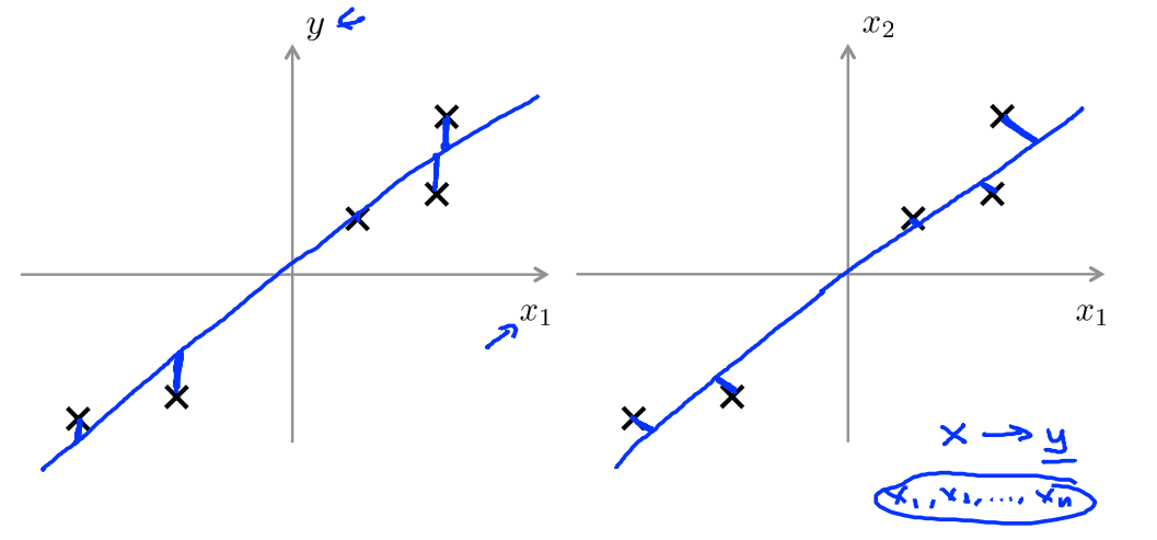
Hypothesis

\[h_\theta=\Theta^Tx=\theta_0x_0+\theta_1x_1+\theta_2x_2+\dots+\theta_nx_n \]

Cost function

\[J(\theta_0,\theta_1,\dots,\theta_n)=\frac{1}{2m}\sum_{i=1}^m(h_\theta(x^{(i)})-y^{(i)}) \]

Gradient descent

\[\theta_j:=\theta_j-\alpha\frac{\partial}{\partial\theta_j}J(\theta_0,\dots,\theta_n) \]

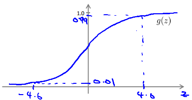
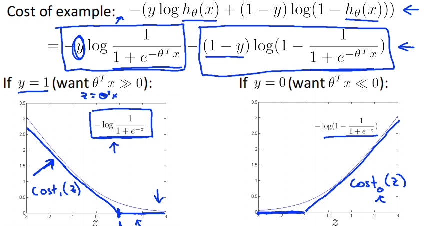
Logistic Regression Model

\[g(x)=\frac{1}{1+e^{-z}} \]

\[h_\theta(x)=g(\theta^Tx)=\frac{1}{1+e^{-\theta^Tx}} \]

Interpretation of Hypothesis Output

\(h_\theta(x)\) estimated probability that y=1 on input x。

Example: If \(x = \left[\begin{matrix}1\\tumorsize\end{matrix}\right]\) and \(h_\theta(x)=0.7\)

This tell patient that 70% chance of tumor being malignant

\[h_\theta(x) = P(y=1|x;\theta) \]

Cost function

\[Cost(h_\theta(x),y) = \begin{cases} -log(h\theta(x)) & if\ y = 1 \\ -log(1-h_\theta(x)) & if\ y = 0 \end{cases} \]

\[Cost = 0\ \ if\ y = 0,h_\theta(x) = 1\\ But\ as\ \ h_\theta(x) \rightarrow 0,Cost\rightarrow\infty \]

\[\begin{align} J(\theta) & = \frac{1}{m}\sum_{i=1}^mCost(h_\theta(x^{(i)}),y^{(i)})\\ & = \frac{1}{m}[\sum_{i=1}^m-y^{(i)}logh_\theta(x^{(i)})-(1-y^{(i)})log(1-h_\theta(x^{(i)}))] \end{align} \]

Gradient Descent

\[\begin{align} \theta_j & = \theta_j - \alpha \frac{\partial}{\partial\theta_j}J(\theta) \\ & = \theta_j -\alpha\sum^m_{i=1}(h_\theta(x^{(i)}) - y^{(i)})x^{(i)}_j \end{align} \]

Lecture7 Regularization

Overfitting : If we have too many features,the learned hypothesis may fit the training set very well,but fail to generalize to new examples(predict prices on new examples)

Addressing overfitting :

1. Reduce numbeer of features
   • Manually select which features to keep
   • Model selection algorithm
2. Regularization
   • Keep all the features,but reduce magnitude/values of parameters \(\theta_j\)
   • Works well when we have a lot of features,each of which contributes a bit to predicting y

Cost function

\[J(\theta) = \frac{1}{2m}[\sum^m_{i=1}(h_\theta(x^{(i)})-y^{(i)})^2 + \lambda \sum^n_{j=1}\theta_j^2] \]

if \(\lambda\) is set to an extremely large value:

• Algorithm works fine; setting \(\lambda\) to be very large can't hurt it
• Algortihm fails to eliminate overfitting.
• Algorithm results in underfitting.(Fails to fit even training data well).
• Gradient descent will fail to converge.

Regularized linear regression

Gradient descent

Repeat{

\[\theta_0:=\theta_0 - \alpha\frac{1}{m}\sum^m_{i=1}(h_\theta(x^{(i)})-y^{(i)})x_0^{(i)} \\ \theta_j:=\theta_j - \alpha[\frac{1}{m}\sum^m_{i=1}(h_\theta(x^{(i)})-y^{(i)})x_j^{(i)} - \frac{\lambda}{m}\theta_j] \]

}

Normal equation

\[\theta=(X^TX+\lambda\underbrace{\left[ \begin{matrix} 0 & 0 & 0 & \cdots & 0 \\ 0 & 1 & 0 & \cdots & 0 \\ 0 & 0 & 1 & \cdots & 0 \\ \vdots & \vdots & \vdots & \ddots & \vdots \\ 0 & 0 & 0 & \cdots & 1 \\ \end{matrix} \right]})^{-1}X^Ty \\(n+1)*(n+1) \]

Regularized logistic regression

Gradient descent

Repeat{

\[\theta_0:=\theta_0 - \alpha\frac{1}{m}\sum^m_{i=1}(h_\theta(x^{(i)})-y^{(i)})x_0^{(i)} \\ \theta_j:=\theta_j - \alpha[\frac{1}{m}\sum^m_{i=1}(h_\theta(x^{(i)})-y^{(i)})x_j^{(i)} - \frac{\lambda}{m}\theta_j] \]

}

Lecture8 Neural NetWork：Representation

Non-linear hypotheses

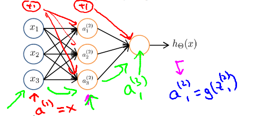
Neural NetWork

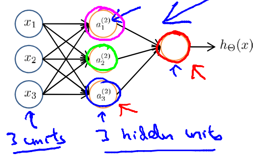
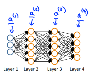
\(a_i^{(j)}\) = "activation" of unit i in layer j

\(\Theta^{(j)}\) = matrix of weights controlling function mapping from layer \(j\) to layer \(j+1\)

\[\begin{align} a_1^{(2)} & = g(\Theta_{10}^{(1)}x_0+\Theta_{11}^{(1)}x_1+\Theta_{12}^{(1)}x_2+\Theta_{13}^{(1)}x_3) \\ a_2^{(2)} & = g(\Theta_{20}^{(1)}x_0+\Theta_{21}^{(1)}x_1+\Theta_{22}^{(1)}x_2+\Theta_{23}^{(1)}x_3) \\ a_1^{(3)} & = g(\Theta_{30}^{(1)}x_0+\Theta_{31}^{(1)}x_1+\Theta_{32}^{(1)}x_2+\Theta_{33}^{(1)}x_3) \\ h_\Theta(x) & = a_1^{(3)}=g(\Theta_{10}^{(2)}a_0^{(2)}+\Theta_{11}^{(2)}a_1^{(2)}+\Theta_{12}^{(2)}a_2^{(2)}+\Theta_{13}^{(2)}a_3^{(2)}) \end{align} \]

if network has \(s_j\) units in layer j,\(s_{j+1}\) units in layer j+1,then \(\Theta^{(j)}\) will be of dimension \(s_{j+1} \times (s_j+1)\)

Vectorized implementation

\[x = \left[\begin{matrix} x_0 \\ x_1 \\ x_3 \\ x_4 \\ \end{matrix}\right] \ z^{(2)} = \left[\begin{matrix} z_1^{(2)} \\ z_2^{(2)} \\ z_3^{(2)} \end{matrix}\right] \\ z^{(2)} = \Theta^{(1)}a^{(1)} \\ a^{(2)} = g(z^{(2)}) \\ Add\ a_0^{(2)} = 1 \Rightarrow a^{(2)} \in \mathbb{R}^4\\ z^{(3)} = \Theta^{(2)})a^{(2)} \\ h_\Theta(x) = a^{(3)} = g(z^{(3)}) \]

Examples and intuitions

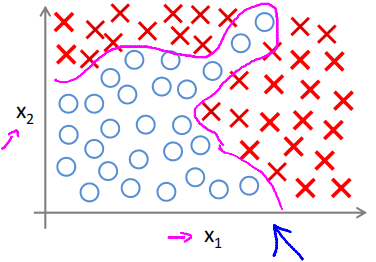
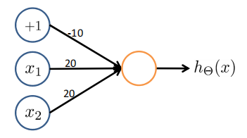
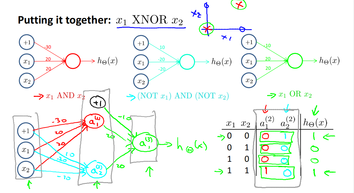
Non-linear classification example: XOR/XNOR

Simple example: AND

\(x_1,x_3 \in {0,1}\)

\(y = x1\ AND\ x_2\)

\[\Theta_{10} = -30 \\ \Theta_{11} = 20 \\ \Theta_{11} = 20 \\ h_\Theta(x) = g(-30 + 20x_1+20x_2) \]

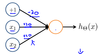
\(x_1\)	\(x_2\)	\(h_\Theta(x)\)
0	0	\(g(-30)\approx0\)
0	1	\(g(-10)\approx0\)
1	0	\(g(-10)\approx0\)
1	1	\(g(10)\approx0\)

Example: OR function

\[h_\Theta(x) = g(-10+20x_1+20x_2) \]

\(x_1\)	\(x_2\)	\(h_\Theta(x)\)
0	0	\(g(-10)\approx0\)
0	1	\(g(10)\approx1\)
1	0	\(g(10)\approx1\)
1	1	\(g(30)\approx1\)

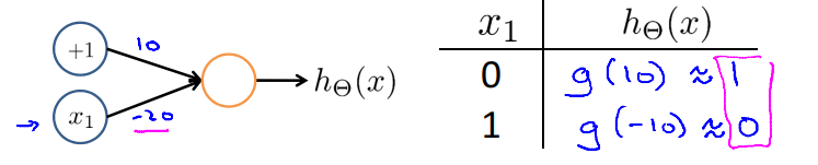
Negation

XOR

Lecture9 Neural Networks:Learning

Cost function

Neural Network (Classifification)

\(L\) = total no. of layer in network

\(S_l\) = no. of units (not counting bias unit) in layer \(l\)

Binary classification

y = 0 or 1 , 1 output unit

Multi-class classification (K classes)

\(y \in \mathbb{R}^K\) e.g. \(\left[\begin{matrix}1\\0\\0\\0\end{matrix}\right]\),\(\left[\begin{matrix}0\\1\\0\\0\end{matrix}\right]\),\(\left[\begin{matrix}0\\0\\1\\0\end{matrix}\right]\),\(\left[\begin{matrix}0\\0\\0\\1\end{matrix}\right]\),K output units

Cost function

logistic regression

\[J(\Theta) = \frac{1}{m}[\sum^m_{i=1} - y^{(i)}\ log(h_\Theta(x^{(i)})) - (1-y^{(i)}) log(1-h_\Theta(x^{(i)}))]+\frac{\lambda}{2m}\sum_{j=1}^n\theta_j^2 \]

Neural network:

\[h_\Theta(x) \in \mathbb{R}^K\ \ (h_\Theta(x))_i = i^{th} output\\ J(\Theta) = \frac{1}{m}[\sum^m_{i=1}\sum_{k=1}^K - y_k^{(i)}\ log(h_\Theta(x^{(i)}))_k - (1-y_k^{(i)}) log(1-h_\Theta(x^{(i)}))_k]+\frac{\lambda}{2m}\sum_{l=1}^{L-1}\sum_{i=1}^{s_l}\sum_{j=1}^{s_l+1}(\theta^{(l)}_{ji})^2 \]

Backpropagation algorithm

Gradient computation

Given one training example(x,y),Forward propagation:

\[\begin{align} a^{(1)} & = x \\ z^{(2)} & = \Theta^{(1)} a^{(1)} \\ a^{(2)} & = g(z^{(2)})\ (add\ a_0^{(2)}) \\ z^{(3)} & = \Theta^{(2)} a^{(2)} \\ a^{(3)} & = g(z^{(3)})\ (add\ a_0^{(3)}) \\ z^{(4)} & = \Theta^{(3)} a^{(3)} \\ a^{(4)} & = h_\Theta(x) = g(z^{(4)}) \\ \end{align} \]

Backpropagation algorithm

Intuition: \(\delta_j^{(l)}\) = "error" of node \(j\) in layer \(l\) ,Formally

\[\delta_j^{(l)} = \frac{\partial}{\partial z_j^{(l)}}J \]

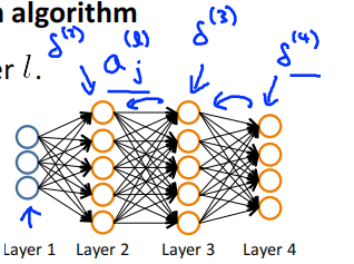
For each output unit (layer L = 4)

\[\begin{align} \delta^{(4)}_j & = a_j^{(4)} - y_j \Rightarrow \delta^{(4)} = a^{(4)}-y\\ \delta^{(3)} & = ((\Theta^{(3)})^T\delta^{(4)}).*g'(z^{(3)})\\ \delta^{(2)} & = ((\Theta^{(2)})^T\delta^{(3)}).*g'(z^{(2)})\\ \\ g'(z^{(3)}) & =a^{(3)}.*(1-a^{(3)})\\ g'(z^{(2)}) & =a^{(2)}.*(1-a^{(2)}) \end{align} \]

Step of Algorithm

set \(\Delta_{ij}^{(l)} = 0\) (for all l,i,j)

For i = 1 to m

​ Set \(a^{(1)} = x^{(i)}\)

​ Perform forward propagation to compute \(a^{(l)}\) for \(l=2,3,\cdots,L\)

​ Using \(y^{(i)}\),compute \(\delta^{(L)} = a^{(L)}-y^{(i)}\)

​ compute \(\delta^{(L-1)},\delta^{(L-2)},\cdots,\delta^{(2)}\)

​ \(\Delta^{(l)}_{ij} += a^{(l)}_j\delta^{(l+1)}_i\)

\(D_{ij}^{(l)} = \frac{1}{m}\Delta_{ij}^{(l)}+\lambda\Theta_{ij}^{(l)}\ \ if\ j \neq 0\)

\(D_{ij}^{(l)} = \frac{1}{m}\Delta_{ij}^{(l)}\ \ if\ j = 0\)

\(\frac{\partial}{\partial\Theta_{ij}^{(l)}}J(\Theta)=D_{ij}^{(l)}\)

Backpropagation intuition

对\(\delta^{(L)} = a^{(L)}-y\)的推导

损失函数选择 交叉熵函数，激活函数选择sigmoid函数。

对于如下图所示的神经网络求$$\delta^{(3)}$$

即对下函数求导。此处选用一个样本作为例子，y为该样本的真实值的向量，z3也为向量。

求导过程如下

\[\begin{align} J_\theta(z_3) = &\sum_{k=1}^{K}-y_k\ log(\frac{1}{1+e^{-z_k^{(3)}}}) - (1-y_k) log(1-\frac{1}{1+e^{-z_k^{(3)}}})\\ J'_\theta(z_k^{(3)})= & -y_k\ (1+e^{-z_k^{(3)}})\frac{-1}{(1+e^{-z_k^{(3)}})^2}e^{-z_k^{(3)}}(-1)-(1-y)\frac{1+e^{-z_k^{(3)}}}{e^{-z_k^{(3)}}}(-1)\frac{-1}{(1+e^{-z_k^{(3)}})^2}e^{-z_k^{(3)}}(-1) \\ = & - \frac{y_ke^{-z_k^{(3)}}}{1+e^{-z_k^{(3)}}} - \frac{y_k-1}{1+e^{-z_k^{(3)}}} \\ = & -\frac{(1+e^{-z_k^{(3)}})y_k-1}{1+e^{-z_k^{(3)}}} \\ = & \frac{1}{1+e^{-z_k^{(3)}}} - y_k \\ = & h_k - y_k \\ = & a^{(3)}_k - y_k \end{align} \]

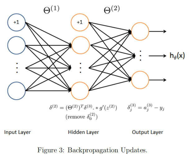
对\(((\Theta^{(l)})^T\delta^{(l+1)})\)的理解

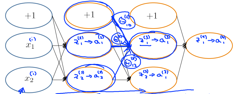
求得\(\delta^{(l+1)}\)之后，要求得\(\delta^{(l)}\)，需要求得\(\frac{\partial}{\partial a^{(l)}}J\)。使用链式法则进行推导

前向传播过程中，\(z_1^{(3)}=\Theta^{(2)}_{10}\times1+\Theta^{(2)}_{11}a^{(2)}_1+\Theta^{(2)}_{12}a^{(2)}_2\)，\(z_2^{(3)}\)同理

所以反向传播时候,\(\frac{\partial}{\partial a_1^{(2)}}J = \Theta_{11}^{(2)} \delta^{(3)}_1 + \Theta_{21}^{(2)} \delta^{(3)}_2\)，\(\frac{\partial}{\partial a_2^{(2)}}J\)同理

所以

\[\frac{\partial}{\partial a^{(l)}}J=((\Theta^{(l)})^T\delta^{(l+1)}) \]

求\(\delta^{(l)}\)时，再次运用链式法则

因为\(a^{(l)}=g(z^{(l)})\)，即\(a_i^{(l)}=\frac{1}{1+e^{(-z^{(l)}_i)}}\)所以

\[\begin{align} \delta^{(l)} &= \frac{\partial}{\partial a^{(l)}}\frac{\partial a^{(l)}}{\partial z^{(l)}}J \\ &= ((\Theta^{(l)})^T\delta^{(l+1)}).*g'(z^{(l)}) \\ &= ((\Theta^{(l)})^T\delta^{(l+1)}).*(a^{(l)}.*(1-a^{(l)})) \end{align} \]

Gradient Checking

gradApprox = (J(theta+EPSILON) - J(theta-EPSILON))/(2*EPSILON)

\(\theta \in \mathbb{R}^n\) (E.g. \(\theta\) is "unrolled" version of \(\theta^{(1)}\), \(\theta^{(2)}\), \(\theta^{(3)}\)）

\[\theta = [\theta_1,\theta_2,\theta_3,\cdots,\theta_n]\\ \frac{\partial}{\partial\theta_1}J(\theta)\approx\frac{J(\theta_1+\epsilon,\theta_2,\theta_3,\cdots,\theta_n)-J(\theta_1-\epsilon,\theta_2,\theta_3,\cdots,\theta_n)}{2\epsilon}\\ \vdots\\ \frac{\partial}{\partial\theta_n}J(\theta)\approx\frac{J(\theta_n,\theta_2,\theta_3,\cdots,\theta_n+\epsilon)-J(\theta_1,\theta_2,\theta_3,\cdots,\theta_n-\epsilon)}{2\epsilon}\\ \]

Random initialization

Zero initialization

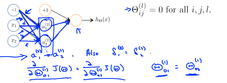
正向传播的时候，\(a_1^{(2)} = a_2^{(2)}\)，所以

\[\delta_1^{(2)}=\delta_2^{(2)}\\ \frac{\partial}{\partial\Theta_{01}^{(1)}}J(\Theta)=\frac{\partial}{\partial\Theta_{01}^{(1)}}J(\Theta)\\ \Theta_{01}^{(1)}=\Theta_{02}^{(1)} \]

After each update,parameters corresponding to inputs going into each of two hidden units are identical

Symmetry breaking

Initialize each \(\Theta_{ij}^{(l)}\) to a random value in \([-\epsilon,\epsilon]\)

Lecture10 Advice for applying machine learning

Train / validation / test error

均不考虑正则化

\[J_{train}(\theta)=\frac{1}{2m}\sum_{i=1}^m(h_\theta(x^{(i)})-y^{(i)})^2\\ J_{cv}(\theta)=\frac{1}{2m_{cv}}\sum_{i=1}^{m_{cv}}(h_\theta(x_{cv}^{(i)})-y_{cv}^{(i)})^2\\ J_{test}(\theta)=\frac{1}{2m_{test}}\sum_{i=1}^{m_{test}}(h_\theta(x_{test}^{(i)})-y_{test}^{(i)})^2 \]

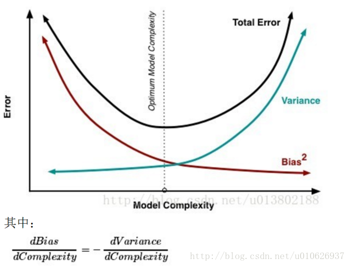
Diagnosing bias vs. variance

偏差： 描述的是预测值（估计值）的期望与真实值之间的差距。偏差越大，越偏离真实数据集。

方差： 描述的是预测值的变化范围，离散程度，也就是离其期望值的距离。方差越大，预测结果数据的分布越散。

用一个参数少的，简单的模型进行预测，会得到低方差，高偏差，通常会出现欠拟合。

理解：简单的模型，对于不同的输出输出的值差不多，变化范围较小，方差就小。输出结果较固定，难以贴近真实值，偏差就高。

用一个参数多的，复杂的模型进行预测，会得到高方差，低偏差，通常出现过拟合。

理解：复杂的模型，能够很好的拟合数据，预测值与真实值更加接近，偏差就小。输出结果易波动，变化范围大，方差就大。

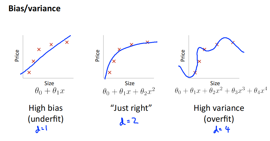
Bias/variance

Lecture11 Machine learning system design

Lecture12 Support Vector Machines

Alternative view of logistic regression

support vector machine:

\[\underset{\theta}{min}C\sum^m_{i=1}[y^{(i)}cost_1(\theta^Tx^{(i)})+(1-y^{(i)})cost_0(\theta^Tx^{(i)})]+\frac{1}{2}\sum^n_{i=1}\theta^2_j \]

hypothesis:

\[h_\theta(x)=\begin{cases} 1 & if\ \theta^Tx\geq0 \\ 0 & otherwise \end{cases} \]

Large Margin Intuition

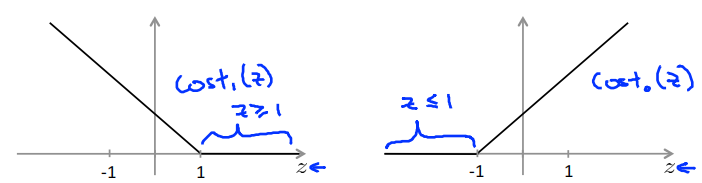
If y = 1,we want \(\theta^Tx\geq1\) (not just \(\geq0\))

If y = 1,we want \(\theta^Tx\leq-1\) (not just \(< 0\))

这里假设SVM的参数C为一个很大的数，比如10w，那么为了使损失函数尽可能的小，就要使得\(\sum^m_{i=1}[y^{(i)}cost_1(\theta^Tx^{(i)})+(1-y^{(i)})cost_0(\theta^Tx^{(i)})]\)尽可能的小，即每个样本都被正确的分类。

在此基础上，也要使\(\frac{1}{2}\sum^n_{i=1}\theta^2_j\)尽可能的小。

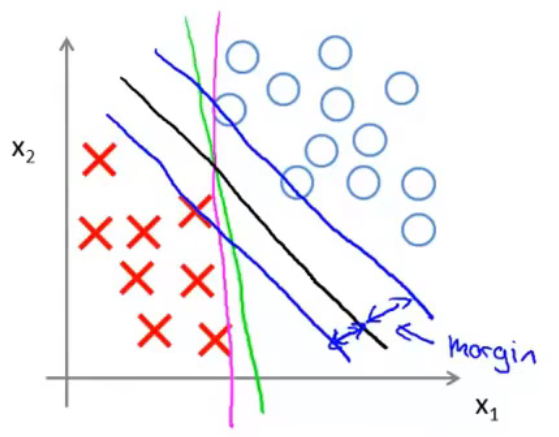
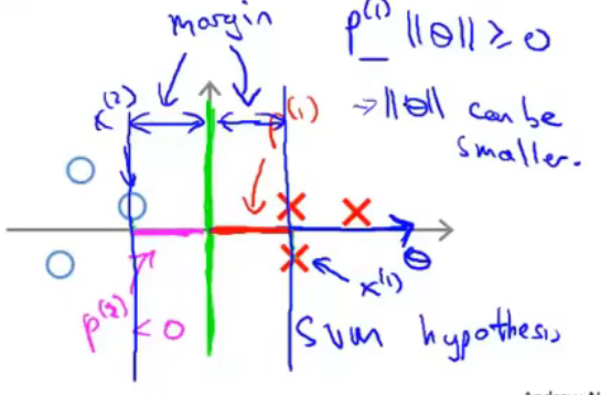
用图来进行表示。尝试用一条线来分隔两类样本。黑线的分隔效果比绿线、紫线的分隔效果更好，因为黑线有着比绿、紫二线更大的margin。此处的margin指的是距离分隔线最近的样本到分隔线的距离（即样本在\(\theta\)向量方向上的投影长度，\(\theta\)向量与分隔线是垂直的，具体见下）。这使得黑线拥有更好的鲁棒性。总而言之，SVM会选择一个模型尽量把正样本和负样本以最大的间距分开。

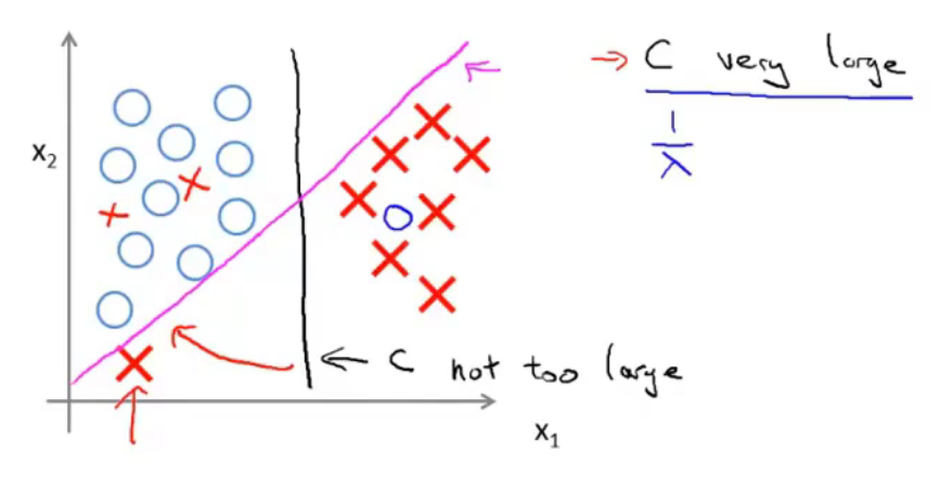
面对下图所示的情况，C较小时，分隔线是黑线。当C设置的非常大的时候，SVM会努力把所有样本都正常分类，分隔线会从黑线移动到紫线。

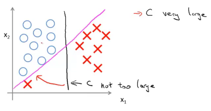
当数据不是线性可分的时候，如果C较小，那么SVM依然能够正常的进行分类。

The mathematics behind large margin classification(optional)

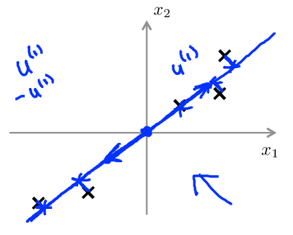
Vector Inner Product

\(u=\left[\begin{matrix}u_1\\u_2\end{matrix}\right]\) , \(v=\left[\begin{matrix}v_1\\v_2\end{matrix}\right]\)

\(\left \|u\right\|\) = length of vector \(u\) = \(\sqrt{u_1^2+u_2^2}\)

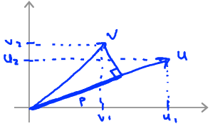
\(p\) = length of projection of \(v\) onto \(u\)

\(u^Tv=p \cdot \left \|u\right\|=u_1v_1+u_2v_2\)

SVM Decision Boundary

这里依旧假设C为一个极大的数，因此要正确的分类每一个数，即损失函数的前一项为0，目标函数变成

\[\underset{\theta}{min}\frac{1}{2}\sum^n_{j=1}\theta^2_j=\frac{1}{2}\left\|\theta\right\| \\ \begin{align} s.t.\ &\theta^Tx^{(i)} \ge 1 & if\ y^{(i)}=1\\ &\theta^Tx^{(i)} \le -1 & if\ y^{(i)}=0 \end{align} \]

此处先假设\(\theta_0=0\)，即\(\theta\)向量经过原点。\(\theta^Tx\)如下图所示。\(\theta^Tx^{(i)}=p^{(i)}\left\|\theta\right\|\)

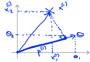
对于如下图所示的数据。绿色的线为分隔线，垂直与向量\(\theta\)。

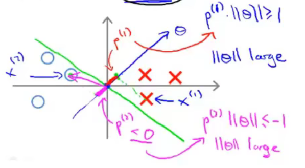
为了使得样本\(x^{(1)}\)被分类到正样本，需要\(\theta^Tx^{(i)}=p^{(i)}\left\|\theta\right\|\ge1\)。与此同时，我们还需要\(\left\|\theta\right\|\)尽可能的小（\(\underset{\theta}{min}\frac{1}{2}\sum^n_{j=1}\theta^2_j=\frac{1}{2}\left\|\theta\right\|\)）。所以我们就需要投影\(p^{(i)}\)尽可能的大，这样\(\left\|\theta\right\|\)就可以尽可能的小。此处的投影长度与前面提到的样本到分隔线的间隔是同一个概念。所以SVM求得的\(\theta\)如下图所示。

总结

SVM的目标函数的前一部分\(\sum^m_{i=1}[y^{(i)}cost_1(\theta^Tx^{(i)})+(1-y^{(i)})cost_0(\theta^Tx^{(i)})]\)的目标是尽量正确的划分每个样本。后面一部分\(\frac{1}{2}\sum^n_{i=1}\theta^2_j\)的目标是\(\theta\)向量的长度尽可能的小，从而使样本在\(\theta\)向量方向上的投影尽可能的大，即样本到分隔线的距离尽可能的大，从而使得SVM模型具有更好的鲁棒性。两者结合，整个函数的目的就是在尽可能正确划分样本的情况下，使模型具有更好的鲁棒性。参数C则是控制两个目标哪个目标更为重要

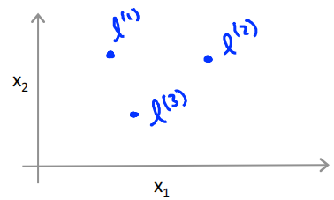
Kernels

Given x,compute new feature depending on proximity to landmarks \(l^{(1)},l^{(2)},l^{(3)}\)

\[f_1=similarity(x,l^{(1)})=exp(-\frac{\left \| x-l^{(1)} \right \|^2}{2\sigma^2})\\ f_1=similarity(x,l^{(2)})=exp(-\frac{\left \| x-l^{(2)} \right \|^2}{2\sigma^2})\\ f_1=similarity(x,l^{(3)})=exp(-\frac{\left \| x-l^{(3)} \right \|^2}{2\sigma^2}) \]

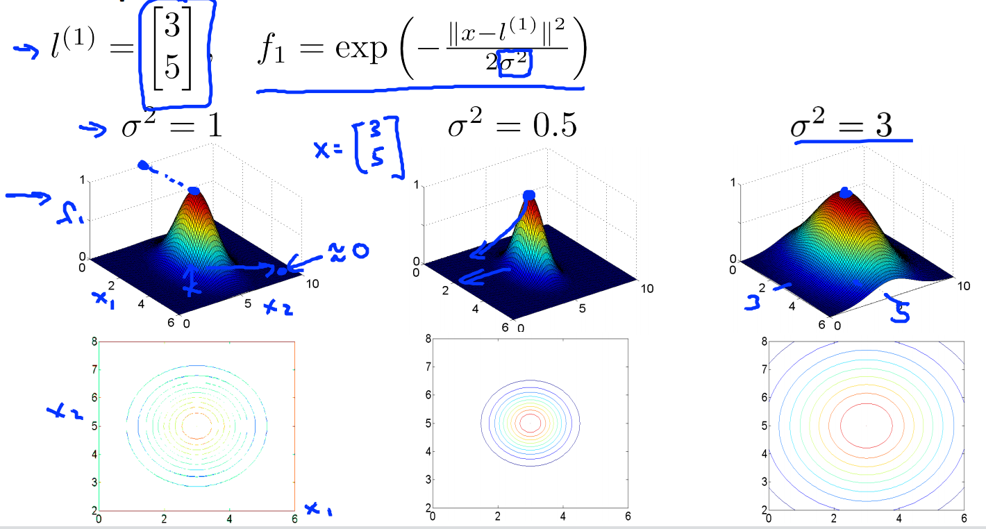
核函数指的就是similitary函数，\(exp(-\frac{\left \| x-l \right \|^2}{2\sigma^2})\)就是高斯核。

当\(x \approx l\) 时，\(f\approx exp(-\frac{0}{2\sigma^2}) \approx1\)

当\(x\)距离\(l\)很远时，\(f\approx exp(-\frac{(large\ number)^2}{2\sigma^2}) \approx0\)

\(\sigma^2\)的大小控制相似函数的平滑程度。\(\sigma^2\)越大，函数越平滑，\(\sigma^2\)越小，函数越陡峭

SVM with Kernels

给定m个样本\((x^{(1)},y^{(1)}),(x^{(2)},y^{(2)}),\cdots,(x^{(m)},y^{(m)})\)，选择每个x作为标记点，即\(l^{(1)}=x^{(1)},l^{(2)}=x^{(2)},\cdots,l^{(m)}=x^{(m)}\)

对于给定的样本x，计算

\[f_1=similarity(x,l^{(1)})\\ f_2=similarity(x,l^{(2)}) \]

输入\(x^{(i)}\)从原来的\(x^{(i)}\in\mathbb{R}^n\)变成了\(f^{(i)}=\left[\begin{matrix}f_0^{(i)}\\f_1^{(i)}\\\vdots\\f_m^{(i)}\end{matrix}\right]\) ，此处\(f_0^{(i)}=1\)，\(f^{(i)} \in\mathbb{R}^{m+1}\)

Hypothesis：Given x,compute features \(f \in \mathbb{R}^{m+1}\),predict "y=1" if \(\theta^Tf=\theta_0f_0+\theta_1f_1+\dots+\theta_mf_m\ge0(\theta\in\mathbb{R}^{m+1})\)

Training:

\[\underset{\theta}{min}C\sum^m_{i=1}[y^{(i)}cost_1(\theta^Tf^{(i)})+(1-y^{(i)})cost_0(\theta^Tf^{(i)})]+\frac{1}{2}\sum^m_{i=1}\theta^2_j \]

最后一项\(\frac{1}{2}\sum^m_{i=1}\theta^2_j\)也可以写作\(\theta^T\theta\)（忽略\(\theta_0\)）。实际实现时最后一项会优化成\(\theta^TM\theta\)，矩阵\(M\)取决于你的核函数，这意味着我们缩小了一种类似的度量，从而使SVM更有效率的运行。

SVM parameters

C偏大，低偏差，高方差，过拟合

C偏小，高偏差，低方差，欠拟合

\(\sigma^2\)偏大，特征\(f_i\)变化平滑，高偏差，低方差，欠拟合

\(\sigma^2\)偏小，特征\(f_i\)变化迅速，低偏差，高方差，过拟合

Lecture 14 Dimensionality Reduction

principal component analysis problem formulation

Reduce from 2-dimension to 1-dimension:Find a direction(a vector \(u^{(1)}\in\mathbb{R}^n\)) onto which to project the data so as to minimize the projection error

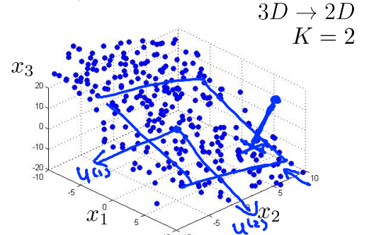
Reduce from n-dimension to k-dimension:Find k vectors \(u^{(1)},u^{(2)},\cdots,u^{(k)}\) onto which to project the data,so as to minimize the projection error.

PCA is not linear regression

linear regression最小化的目标函数是：样本的预测值和真实值之间误差的均方和

PCA最小化的目标函数是：样本到分界线（面）的投影距离的均方和

Principal Component Analysis algorithm

Data preprocessing

Training set:\(x^{(1)},x^{(2)},\dots,x^{(m)}\)

feature casling/mean normalization

\[x_j=\frac{x_j-\mu_j}{s_j} \]

Principal Component Analysis(PCA) algorithm

Reduce data from n-dimensions to k-dimensions

Compute "covariance matrix":

\[\Sigma=\frac{1}{m}\sum_{i=1}^n(x^{(i)})(x^{(i)})^T\\ \]

此处\(\Sigma\in\mathbb{R}^{n\times n}\)

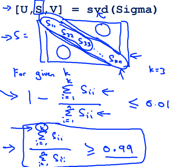
Compute "eigenvector" of matrix \(\Sigma\):

\[[U,S,V]=svd(\Sigma)\\ U=\left[\begin{matrix}u^{(1)},u^{(2)},\cdots,u^{(n)}\end{matrix}\right] \]

此处\(U\in\mathbb{R}^{n\times n}\)

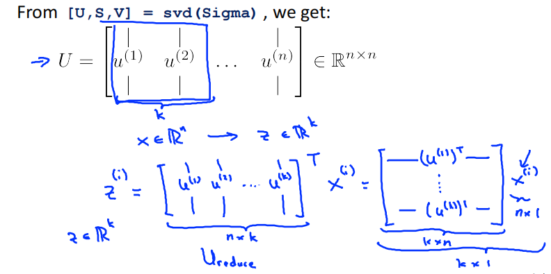
选择\(U\)的前k列向量来进行压缩

\[z^{(i)} = \underset{n\times k}{\underbrace{\left[\begin{matrix}u^{(1)},u^{(2)},\dots,u^{(k)}\end{matrix}\right]}}^Tx^{(i)} =\underset{k\times 1}{\underbrace{\underset{k\times n}{\underbrace{\left[\begin{matrix}(u^{(1)})^T\\(u^{(2)})^T\\\vdots\\(u^{(k)})^T\end{matrix}\right]}}\underset{n\times 1}{\underbrace{x^{(i)}}}}} \]

\(U_{reduce}^T\)指\(\underset{n\times k}{\underbrace{\left[\begin{matrix}u^{(1)},u^{(2)},\dots,u^{(k)}\end{matrix}\right]}}\)这个矩阵

Reconstruction from compressed representation

\[x^{(i)}=U_{reduce}z^{(i)} \]

Choosing the number of prinvipal components

Choosing k(number of pricipal components)

Average squared projection error:\(\frac{1}{m}\sum_{i=1}^m\left\|x^{(i)}-x_{approx}^{(i)}\right\|^2\)

Total variation in the data:\(\frac{1}{m}\left\|x^{(i)}\right\|^2\)

Typically,choose \(k\) to be smallest value so that

\[\frac{\frac{1}{m}\sum^m_{i=1}\left\|x^{(i)}-x_{aprrox}^{(i)}\right\|^2}{\frac{1}{m}\left\|x^{(i)}\right\|^2}\leq0.01\ (1\%) \]

"99%" of variance is retained

somtimes,0.01 can be

Sometimes 0.01 can be replaced by 0.05 or 0.1,which means 95% or 90% of variance is retained.

Algorithm:

Try PCA with k = 1,k = 2,k = 3...

compute \(U_{reduce},z^{(1)},z^{(2)},\dots,z^{(m)},x_{approx}^{(1)},x_{approx}^{(2)},\dots,x_{approx}^{(m)}\)

check if

\[\frac{\frac{1}{m}\sum^m_{i=1}\left\|x^{(i)}-x_{aprrox}^{(i)}\right\|^2}{\frac{1}{m}\left\|x^{(i)}\right\|^2}\leq0.01 \]

We can also use the method shown below

Advice for applying PCA

Supervised learning speedup

\((x^{(1)},y^{(1)}),(x^{(2)},y^{(2)}),\dots,(x^{(m)},y^{(m)})\)

Extract inputs:

Unlabeled dataset:

\[x^{(1)},x^{(2)},\dots,x^{(m)}\in\mathbb{R}^{10000}\\ \downarrow PCA\\ z^{(1)},z^{(2)},\dots,z^{(m)}\in\mathbb{R}^{1000} \]

New training set:\((z^{(1)},y^{(1)}),(z^{(2)},y^{(2)}),\dots,(z^{(m)},y^{(m)})\)

Note:Mapping \(x^{(i)}\rightarrow z^{(i)}\) should be defined by running PCA only on the training set.This mapping can be applied as well to the examples \(x^{(i)}_{cv}\) ans \(x^{(i)}_{test}\) in the cross validation and test sets

Application of PCA

• Compression (Choose k by % of variance retained)
  • Reduce memory/disk needed to store data
  • Speed up learning algorithm
• Visualization (k = 2 or k = 3)

Bad use of PCA:To prevent overfitting

Use \(z^{(i)}\) instead of \(x^{(i)}\) to reduce the number of features to \(k<n\)

Thus,fewer features,less likely to overfit

This might work OK,but isn't a good way to address overfitting.Use regularization instead.

\[\underset{\theta}{min}\frac{1}{2m}\sum_{i=1}^m(h_\theta(x^{(i)})-y^{(i)})^2+\frac{\lambda}{2m}\sum_{j=1}^n\theta_j^2 \]

PCA is sometimes used where it shouldn't be

Design of ML system:

• Get training set\(\{(x^{(1)},y^{(1)}),(x^{(2)},y^{(2)}),\dots,(x^{(m)},y^{(m)})\}\)
• Run PCA to reduce \(x^{(i)}\) in dimension to get \(z^{(i)}\)
• Train logistic regression on \(\{(z^{(1)},y^{(1)}),\dots,(z^{(m)},y^{(m)})\}\)
• Test on test set:Map \(x_{test}^{(i)}\) to \(z_{test}^{(i)}\).Run \(h_\theta(z)\) on \(\{(z^{(1)},y^{(1)}),\dots,(z^{(m)},y^{(m)})\}\)

How about doing the whole thing without using PCA?

Before implementing PCA,first try running whatever you want to do with the original/raw data \(x^{(i)}\).Only if that doesn't do what you want,the implement PCA and consider using \(z^{(i)}\)

Lecture 15 Anomaly detection

problem motivation

Gaussian distribution

Algorithm

Density estimation

Training set : \({x^{(1)},x^{(2)},\dots,x^{(m)}}\)

Each example is \(x \in \mathbb{R}^n\)

\[x_1 \sim N(u_1,\sigma_1^2)\\ x_2 \sim N(u_2,\sigma_2^2)\\ \vdots\\ x_n \sim N(u_n,\sigma_n^2)\\ p(x) = p(x_1,u_1,\sigma_1^2)p(x_2,u_2,\sigma_2^2)\dots p(x_n,u_n,\sigma_n^2) =\prod_{j=1}^p(x_j,u_j,\sigma_j^2) \]

Anomaly detection algorithm

1. Choose features \(x_i\) that you think might be indicative of anomalous example

2. Fit parameters \(u_1,u_2,\dots,u_n,\sigma_1^2,\sigma_2^2,\dots,\sigma_n^2\)

   \(u_j=\frac{1}{m}\sum_{i=1}^mx_j^{(i)}\)

   \(\sigma_j^2=\frac{1}{m}\sum_{i=1}^m(x_j^{(i)}-u_j)^2\)

3. Given new example \(x\),compute \(p(x)\)

   \[p(x)=\prod_{j=1}^np(x_j,u_j,\sigma_j^2)=\prod_{j=1}^n\frac{1}{\sqrt{2\pi}\sigma_j}exp(-\frac{(x_j-u_j)^2}{2\sigma^2_j}) \]

   Anomaly if \(p(x)<\varepsilon\)

Anomaly detection example

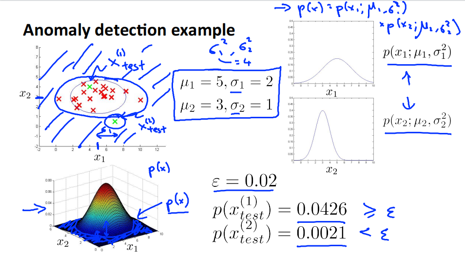
\(x_1\sim N(5,4)\)，\(x_2\sim N(3,1)\)

对于测试样本\(x_{test}^{(1)}\)，其坐标为\((a,b)\)，计算其落在横坐标\(a\)上的概率\(p(a,u_1,\sigma_1^2)\)，落在纵坐标\(b\)上的概率\(p(b,u_2,\sigma_2^2)\)。\(p(x) = p(a,u_1,\sigma_1^2)p(b,u_2,\sigma_2^2)\)就是测试样本\(x_{test}^{(1)}\)落在平面上点\((a,b)\)的概率。因为\(p(x_{test}^{(1)})=0.0426 \geq \varepsilon\) 所以判定其为正常样本。

同理，\(p(x_{test}^{(2)})=0.0021 \leq \varepsilon\) 所以判定其为异常样本

Developing and evaluating an anomaly detection system

The inportance of real-number evaluation

When developing a learning algorithm (choosing features,etc.),making decisions is much easier if we have a way of evaluating our learning algorithm

Assume we have some labeld data,of anomalous and non-anomalous example(y = 0 if normal,y = 1 if anomalous)

Training set:\(x^{(1)},x^{(2)},\dots,x^{(m)}\) (assume normal examples/not anomalous).把训练集是正常样本的集合，即使溜进了一些异常样本。

Cross validation set: \((x_{cv}^{(1)},y_{cv}^{(1)}),\dots,(x_{cv}^{(m_{cv})},y_{cv}^{(m_{cv})})\)

Test set : \({(x_{test}^{(1)},y_{test}^{(1)}),\dots,(x_{test}^{(m_{test})},y_{test}^{(m_{test})})}\)

验证集和测试集都包含一些异常样本

Aircraft engines motivating example

10000 good (normal) engines

20 flawd engines (anomalous)

Training set : 6000 good engines (y = 0)

CV : 2000 good engines (y = 0),10 anomalous (y = 1)

Test : 2000 good engines (y = 0),10 anomalous (y = 1)

Alternative : （不推荐）

Training set : 6000 good engines (y = 0)

CV : 4000 good engines (y = 0),10 anomalous (y = 1)

Test : 4000 good engines (y = 0),10 anomalous (y = 1)

验证集和测试集应当是两个完全不同的数据集。

Algorithm evaluation

Fit model \(p(x)\) on training set \(\{x^{(1)},\dots,x^{(m)}\}\)

On a cross validation/test example \(x\),predict

\[y = \begin{cases} 1 & if\ p(x)<\varepsilon\ (anomaly)\\ 0 & if\ p(x)\geq\varepsilon\ (normal) \end{cases} \]

possible evaluation metrics:

• True positive,false positive,false negative,true negative
• Precision/Recall
• \(F_1\)-score

Can also use cross validation set to choose parameter \(\varepsilon\)

尝试许多不同的 \(\varepsilon\)，找到使得\(F_1\)-score最大的\(\varepsilon\)

Anomaly detection vs. supervised learning

Anomaly detection	Supervised learning
vary small number of positive example (y = 1).(0-20 is common) Large number of negative (y = 0) examples	Laege number of positive and negative examples
Many different “types" of anomalies.Hard for any algorithm to learn from positive examples what the anomalies look like ; future anomalies may look nothing like any of the anomalous examples we've seen so far	Ecough positive examples for algorithm to get a sense of what positive examples are like,future positive examples likely to be similar to ones in training set

异常检测适用于正样本少，负样本多的情况。监督学习适用于正负样本都多的情况。

异常有很多种，异常样本较少，很难从正样本中学习异常。而且将来出现的异常很可能会与已有的截然不同。适用于异常检测。

监督学习拥有足够多的正样本去学习异常，而且将来出现的异常与当前训练集中的正样本相似。适用于监督学习。

关键是正样本的数量。

Anomaly detection	Supervised learning
Frad detection	Email spam classification
Manufacturing (e.g. aircraft engines)	Wheater prediction
Monitoring machines in a data center	Cancer classification

Choosing what features to use

Non-gaussian features

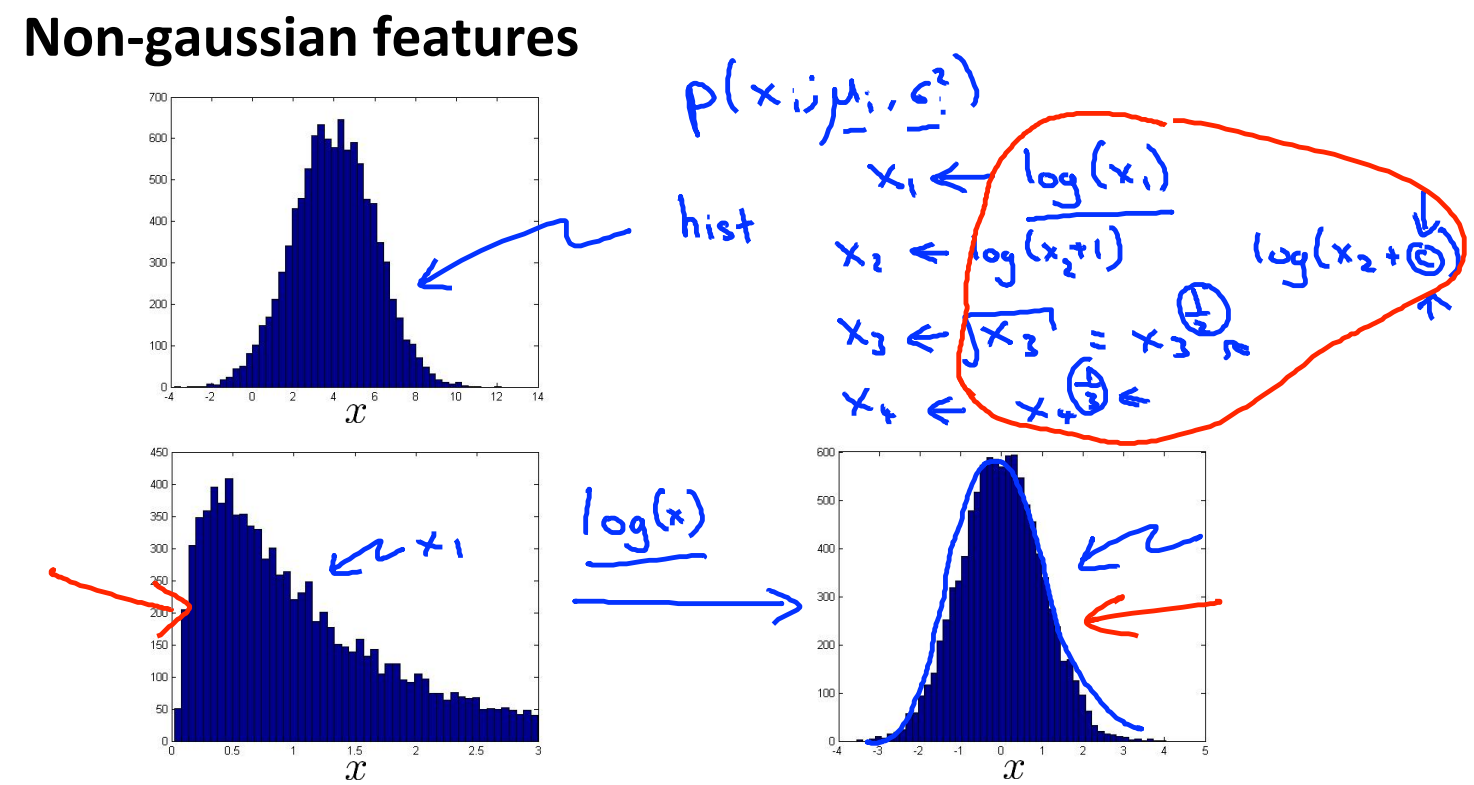
对于不符合高斯分布的数据，通过对数据进行一些转换，使得它看上去更接近高斯分布。虽然不进行转换算法也可以运行，但转换之后，算法可以运行的更好。

通常的转换方式有

\[\begin{align} & x_1 \leftarrow log(x_1)\\ & x_2 \leftarrow log(x_2 + c)\\ & x_3 \leftarrow \sqrt{x_3}\\ & x_4 \leftarrow x_4^{\frac{1}{3}} \end{align} \]

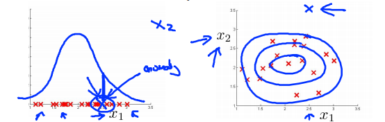
Error analysis for anomaly detection

Want \(p(x)\) large for normal examples \(x\)

​ \(p(x)\) small for anomalous examples \(x\)

Most common problem : \(p(x)\) is comparable (say,both large) for normal and anomalous examples.

发现一个新的特征\(x_2\)，他能够将异常样本和正常样本区分开来。

Monitoring computers in a data center

Choose features that might take on unusually large or small values in the event of an anomaly

\(x_1\)=memory use of computer

\(x_2\)=number of disk accesses/sec

\(x_3\)=CPU load

\(x_4\)=network traffic

\(x_5\)=CPU load / network traffic

\(x_6\)=(CPu load)^2 / network traffic

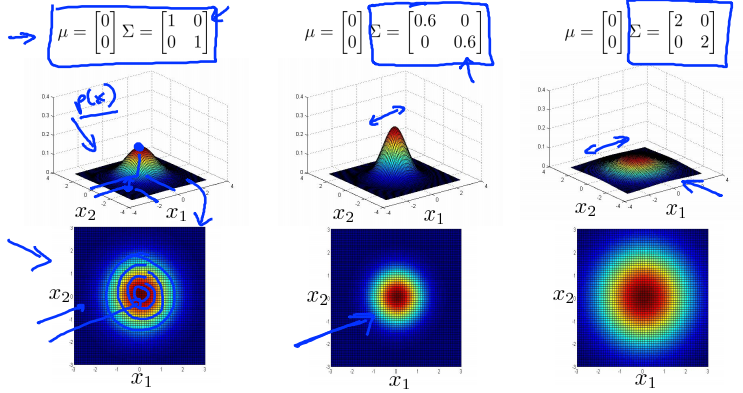
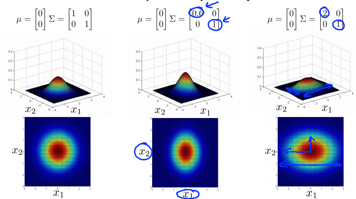
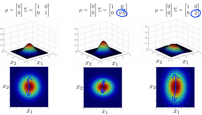
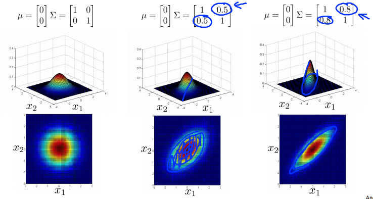
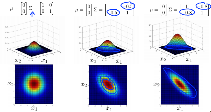
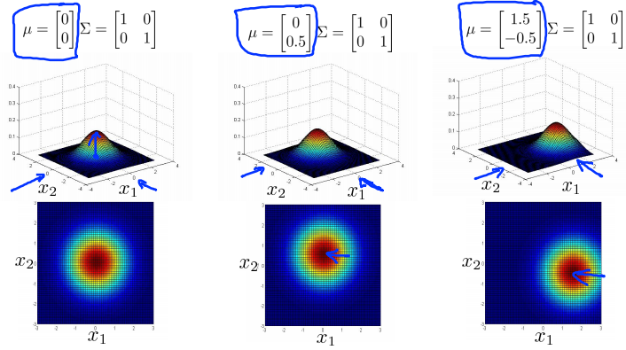
Multivariate Gaussian distribution

Motivating example:Monitoring machines in a data center

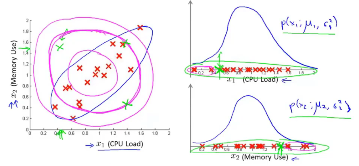
对于绿色样本\(x^{(1)}(0.5,1.5)\)，CPU负载很低，但内存使用量很高，是一个异常样本。如果认为两个变量线性无关，计算结果\(p(x^{(1)})=p(x_1^{(1)},u_1,\sigma_1^2)p(x_2^{(1)},u_2,\sigma_2^2)\)并不低，所以可能不会被归类为异常样本。紫红色的等高线图表示其概率在平面上的分布。但是CPU负载和内存使用量之间存在线性关系。其概率分布是椭圆形的。

Multivariate Gaussian (Normal) distribution

\(x\in\mathbb{R}^n\). Don't model \(p(x_1),p(x_2),\dots\),etc. separately.

Model \(p(x)\) all in one go.

Parameters : \(u \in \mathbb{R}^n\),\(\Sigma \in \mathbb{R}^{n\times n}\)(covariance matrix)

\[p(x;u,\Sigma)=\frac{1}{(2\pi)^{(n/2)}|\Sigma|^{\frac{1}{2}}}exp(-\frac{1}{2}(x-u)^T\Sigma^{-1}(x-u)) \]

Parameter fitting:

Given training set \(\{x^{(1)},x^{(2)},\dots,x^{(m)}\}\)

\[u=\frac{1}{m}\sum_{i=1}^mx^{(i)}\ \ \Sigma=\frac{1}{m}\sum_{i=1}^m(x^{(i)}-u)(x^{(i)}-u)^T \]

Multivariance Gaussian (Normal) examples

Anomaly detection using the multivariance Gaussian distribution

Relationship to origin model

Original model : \(p(x) = p(x_1,u_1,\sigma_1^2)p(x_2,u_2,\sigma_2^2)\dots p(x_n,u_n,\sigma_n^2)\)

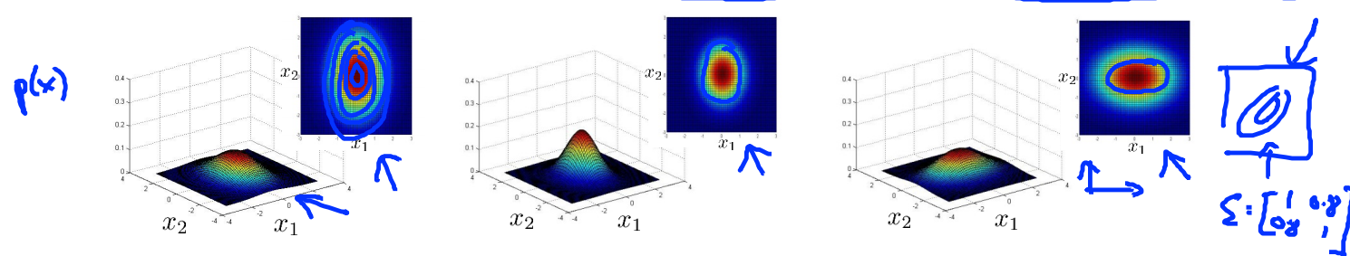
Corresponds to multivariate Gaussian

\[p(x;u,\Sigma)=\frac{1}{(2\pi)^{(n/2)}|\Sigma|^{\frac{1}{2}}}exp(-\frac{1}{2}(x-u)^T\Sigma^{-1}(x-u)) \]

Where \(\Sigma = \left[\begin{matrix}\sigma^2_1&0&\cdots&0\\0&\sigma^2_2&\cdots&0\\\vdots&\vdots&\ddots&\vdots\\0&0&\cdots&\sigma^2_n\end{matrix}\right]\)

原模型的等高线图总是轴对齐的 (axis-aligned)。（变量之间线性无关。）

Original model	Multivariate Gaussian
Manually create features to capture anomalies where \(x_1,x_2\) take unusual combinations of values.e.g.\(x_3=\frac{x_1}{x_2}=\frac{CPU\ load}{memory}\)	Automaticlly capture correlations between features
Computationally cheaper(alternatively,scales better to large)	Computationally more expensive
OK even if \(m\) (training set size) is small	Must have \(m>n\) or else \(\Sigma\) is non-invertible (\(m \geq 10n\))

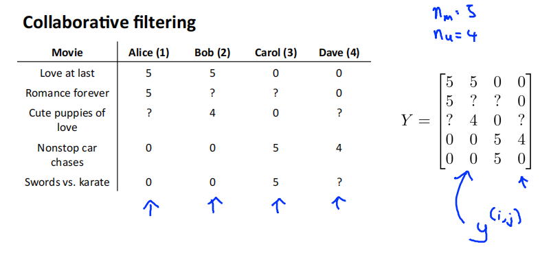
Lecture16 Recommender Systems

Problem formulation

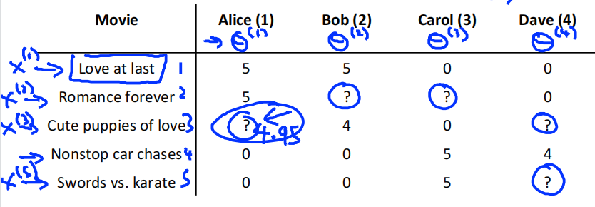
Example:Predicting movie ratings

User rates movies using zero to five stars

\(n_u\) = no. users

\(n_m\) = no.movies

\(r(i,j)\) = 1 if user \(j\) has rated movie \(i\)

\(y(i,j)\) = rating given by user \(j\) to movie \(i\) (defined only if \(r(i,j) = 1\))

Content-based recommendations

Content-based recommender systems

For each user \(j\) ,learn a parameter \(\theta^{(j)}\in\mathbb{R}^3\).Predict user \(j\) as rating movies \((\theta^{(j)})^Tx^{(i)}\)

\(\theta^{(j)}\) = parameter vector for user \(j\) (\(\theta^{(j)}\in\mathbb{R}^{n+1}\))
\(x^{(i)}\) = feature vector for movie \(i\)

For user \(j\) , movie \(i\) ,predicted rating : \((\theta^{(j)})^Tx^{(i)}\)

\(m^{(j)}\) = no. of movies rated by user \(j\)

上图样本中的电影分为两种，前三部是爱情电影，后两部为动作电影。假设电影有两个特征值，第三个电影的特征值为\(x^{(3)}=\left[\begin{matrix}1\\0.9\\0\end{matrix}\right]\)，其中\(x^{(3)}_0\)为偏置，0.9表明该电影偏向爱情电影。用户1对两部爱情电影打分5，对两部动作电影打分0，通过学习得到的用户1的\(\theta^{(3)}=\left[\begin{matrix}0\\5\\0\end{matrix}\right]\)。\((\theta^{(1)})^Tx^{(3)}=5*0.99=4.95\)。所以预测用户1给第三部电影打分为4.95分

Optimization objective

To learn \(\theta^{(j)}\) (parameter for user \(j\)):

\[\underset{\theta^{(j)}}{min}\frac{1}{2}\sum_{i:r(i,j)=1}((\theta^{(j)})^Tx^{(i)} - y^{(i,j)})^2+\frac{\lambda}{2}\sum_{k=1}^n(\theta^{(j)}_k)^2 \]

To learn \(\theta^{(1)},\theta^{(2)},\dots,\theta^{(n_u)}\)

\[\underset{\theta^{(1)},\dots,\theta^{(n_u)}}{min}\frac{1}{2}\sum_{j=1}^{n_u}\sum_{i:r(i,j)=1}((\theta^{(j)})^Tx^{(i)} - y^{(i,j)})^2+\frac{\lambda}{2}\sum_{j=1}^{n_u}\sum_{k=1}^n(\theta^{(j)}_k)^2 \]

Gradient descent update:

\[\theta_k^{(j)}=\theta_k^{(j)} - \alpha\sum_{i:r(i,j)=1}((\theta^{(j)})^Tx^{(i)} - y^{(i,j)})x_k^{(i)}\ \ \ \ (for\ \ k=0) \]

\[\theta_k^{(j)}=\theta_k^{(j)} - \alpha(\sum_{i:r(i,j)=1}((\theta^{(j)})^Tx^{(i)} - y^{(i,j)})x_k^{(i)}+\lambda\theta_k^{(j)})\ \ \ \ (for\ \ k\neq0) \]

Collaborative filtering

协同过滤。该算法有一个有趣的特征，叫做特征学习，即这种算法能够自行学习所需要使用的特征。

problem motivation

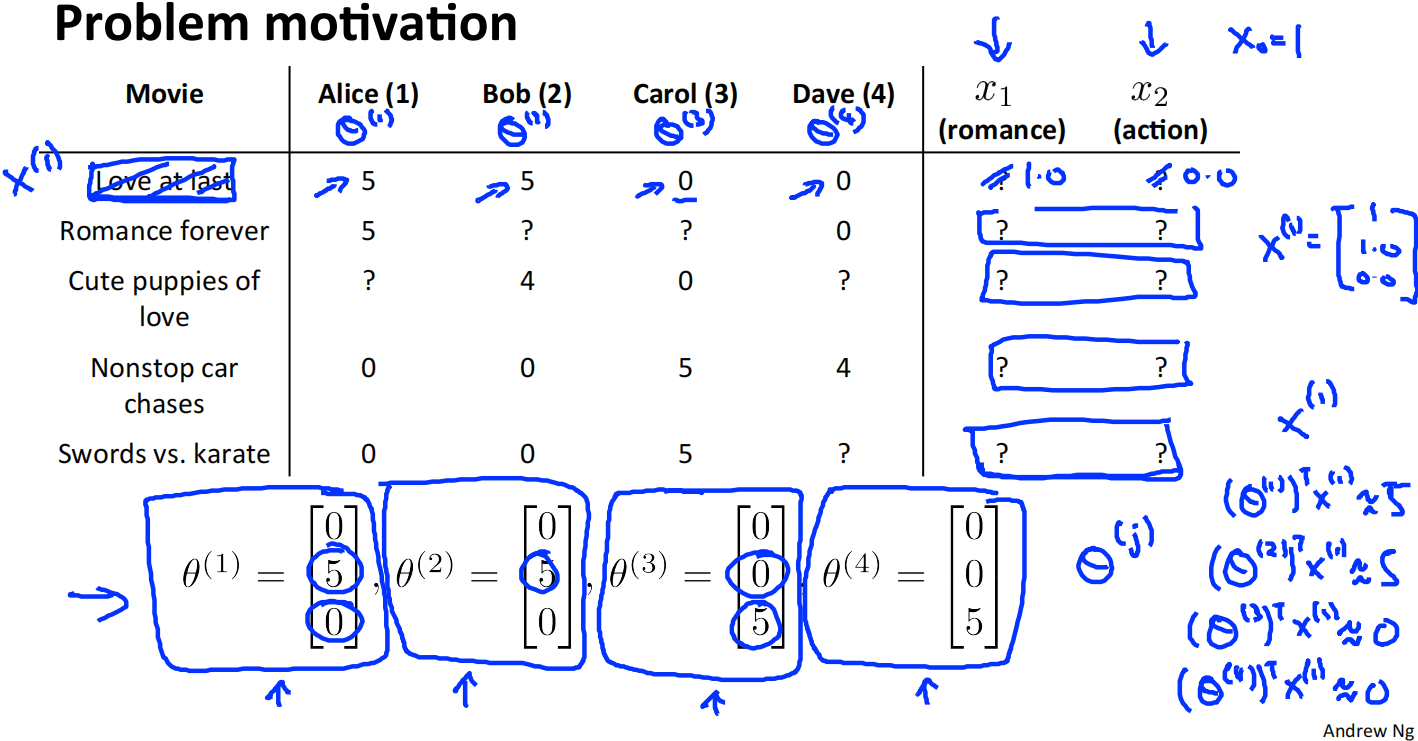
对于该数据集，我们不知道每个电影的特征值，但是知道每个用户的喜好，即图中的\(\theta\)表示。我们可以由此推测出每个电影的特征值。

\[(\theta^{(1)})^Tx^{(1)} \approx 5 \\ (\theta^{(2)})^Tx^{(1)} \approx 5 \\ (\theta^{(3)})^Tx^{(1)} \approx 0 \\ (\theta^{(4)})^Tx^{(1)} \approx 0 \]

由此可知\(x^{(1)}=\left[\begin{matrix}1\\1\\0\end{matrix}\right]\)。其中\(x_0^{(1)}\)是截距项。

Optimization algorithm

Given \(\theta^{(1)},\dots,\theta^{(n_u)}\) , to learn \(x^{(i)}\)

\[\underset{x^{(i)}}{min}\frac{1}{2}\sum_{j:r(i,j)=1}((\theta^{(j)})^Tx^{(i)} - y^{(i,j)})^2+\frac{\lambda}{2}\sum_{k=1}^n(x^{(i)}_k)^2 \]

Given \(\theta^{(1)},\dots,\theta^{(n_u)}\) , to learn \(x^{(1)},\dots,x^{(n_m)}\)

\[\underset{x^{(i)},\dots,x^{(n_m)}}{min}\frac{1}{2}\sum_{i=1}^{n_m}\sum_{j:r(i,j)=1}((\theta^{(j)})^Tx^{(i)} - y^{(i,j)})^2+\frac{\lambda}{2}\sum_{i=1}^{n_m}\sum_{k=1}^n(x^{(i)}_k)^2 \]

Collaborative filtering

Given \(x^{(1)},\dots,x^{(n_m)}\) (and movies ratings),can estimate \(\theta^{(1)},\dots,\theta^{(n_m)}\)

Given \(\theta^{(1)},\dots,\theta^{(n_m)}\) (and movies ratings),can estimate \(x^{(1)},\dots,x^{(n_m)}\)

随机猜一些\(\theta\)，学习出不同电影的特征，再用通过特征来获得一个更好的对参数\(\theta\)的估计，再通过\(\theta\)来获得更好的特征，不断进行迭代，最后收敛到合理的电影特征和合理的对不同用户的参数的估计。

这是基础的协同过滤算法。对于该问题，对于推荐系统来说，该算法得以实现的基础是每个用户都对数个电影进行了评价，并且每个电影都被数位用户评价过，才能重复这个迭代过程来估计 \(x\) 和 \(\theta\)。

当你运行算法时，需要观察大量的用户，观察这些用户的实际动作来协同获得更佳的每个人对电影的评分。

每个用户都对电影做出了评价，每个用户都在帮助算法学习出更合适的特征。学习出来的特征又可以被用来更好地预测其他用户的评分。这是协同的另一个意思，是说每个用户都在帮助算法更好地进行特征学习。

The term collaborative filtering refers to the observation that when you run this algorithm with a large set of users,what all of these users are effectively doing are sort of collaborating to get better movies ratings for everyone because with every user rating some subset of the movies,every user is helping the algorithm a little bit to learn better features,and then by helping by rating a few movies myself,I will be helping the system learn better features and the these features can be used by the system to make better movies predictions for everyone else.And so there is a sense of collaboriation where every user is helping the system learn better for the common good

Collaborative filtering algorithm

Collaborative filtering optimization objective

Minimizing \(x^{(1)},\dots,x^{(n_m)}\) and \(\theta^{(1)},\dots,\theta^{(n_u)}\) simultaneously

\[J(x^{(1)},\dots,x^{(n_m)},\theta^{(1)},\dots,\theta^{(n_u)})=\frac{1}{2}\sum_{(i,j):r(i,j)=1}((\theta^{(j)})^Tx^{(i)}-y^{(i,j)})^2+\frac{\lambda}{2}\sum_{i=1}^{n_m}\sum_{k=1}^n(x^{(i)}_k)^2+\frac{\lambda}{2}\sum_{j=1}^{n_u}\sum_{k=1}^n(\theta^{(j)}_k)^2 \]

Collaborative filtering algorithm

1. Initialize \(x^{(1)},\dots,x^{(n_m)}\) and \(\theta^{(1)},\dots,\theta^{(n_u)}\) to small random values

2. Minimize \(x^{(1)},\dots,x^{(n_m)}\) and \(\theta^{(1)},\dots,\theta^{(n_u)}\) using gradient descent (or an advanced optimization algorithm) E.g. for every \(j = 1,\dots,n_u,i = 1,\dots,n_m\)

   \[x_k^{(j)}=x_k^{(j)} - \alpha(\sum_{j:r(i,j)=1}((\theta^{(j)})^Tx^{(i)} - y^{(i,j)})\theta_k^{(j)}+\lambda x_k^{(j)})\\ \theta_k^{(j)}=\theta_k^{(j)} - \alpha(\sum_{i:r(i,j)=1}((\theta^{(j)})^Tx^{(i)} - y^{(i,j)})x_k^{(i)}+\lambda\theta_k^{(j)}) \]

3. for a user with parameters \(\theta\) and movie with (learned) features \(x\) ,predict a star rating of \(\theta^Tx\)

Vectorization:Low rank matrix factorization

Collaborative filtering

用户对电影的评分用矩阵Y进行表示。

预测评分矩阵：

\[X\Theta^T=\left[ \begin{matrix} --(X^{(1)})^T-- \\ --(X^{(2)})^T-- \\ \vdots \\ --(X^{(n_m)})^T-- \\ \end{matrix} \right] \left[ \begin{matrix} --(\theta^{(1)})^T-- \\ --(\theta^{(2)})^T-- \\ \vdots \\ --(\theta^{(n_u)})^T-- \\ \end{matrix} \right]^T =\left[ \begin{matrix} (\theta^{(1)})^Tx^{(1)} & (\theta^{(2)})^Tx^{(1)} & \cdots & (\theta^{(n_u)})^Tx^{(1)} \\ (\theta^{(1)})^Tx^{(2)} & (\theta^{(2)})^Tx^{(2)} & \cdots & (\theta^{(n_u)})^Tx^{(2)} \\ \vdots & \vdots & \ddots & \vdots \\ (\theta^{(1)})^Tx^{(n_m)} & (\theta^{(2)})^Tx^{(n_m)} & \cdots & (\theta^{(n_u)})^Tx^{(n_m)} \end{matrix} \right] \]

finding related movies

For each product \(i\),we learn a feature vector \(x^{(i)} \in \mathbb{R}^n\)

How to find movies related to movie \(i\)?

small \(\left \|x^{(i)} - x^{(j)} \right \|\) means that movie \(j\) and movie \(i\) are "similar"

5 most similar movies to movie \(i\) : Find the 5 movies j with the smallest \(\left \|x^{(i)} - x^{(j)} \right \|\)

Implementational detail : Mean normalization

Users who have not rated any movies

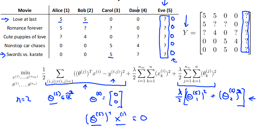
学习5号用户Eve的参数向量\(\theta^{(5)}\)。用户Eve没有评价过任何电影，所以只有\(\frac{\lambda}{2}\sum_{j=1}^{n_u}\sum_{k=1}^n(\theta^{(j)}_k)^2\)这一项对损失函数有影响。为了最小化损失函数，\(\theta^{(5)}=\left[\begin{matrix}0\\0\\0\end{matrix}\right]\)。所以\((\theta^{(5)})^Tx^{(1)} = 0\)，即Eve对每个电影打的分数都是0分。这种结果是存在问题的。

Mean normalization

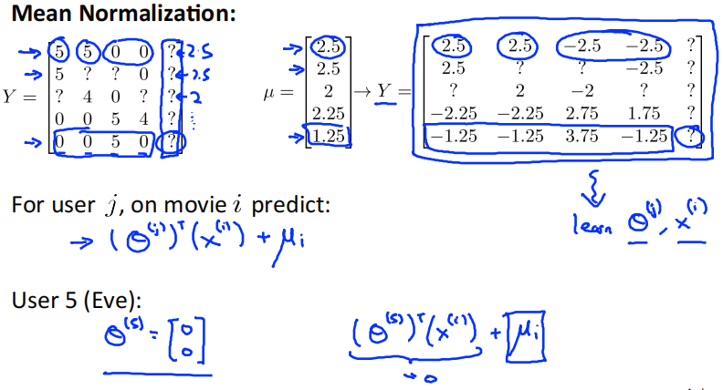
计算出每部电影的平均值，Y减去均值。用新的Y来训练\(\theta^{(i)},x^{(i)}\)。因为用户5仍然没有评价过任何电影，所以问题仍然存在

对于用户 \(j\) 评价电影 \(i\) 时，预测值再加上均值 \(u_i\)。即使预测值为0，得到就是电影的平均分。

Lecture18 Application example:Photo OCR

Problem description and pipeline

The Photo OCR problem

全称：Photo Optical Character Recognition。如何让计算机读出图片中的文字信息

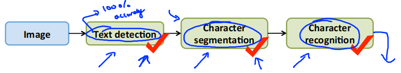
Photo OCR pipeline

1. Text detection

   

2. Character segmentation

   

3. Character classification

   

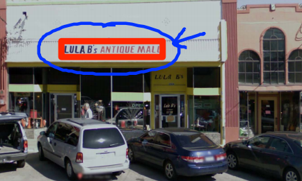
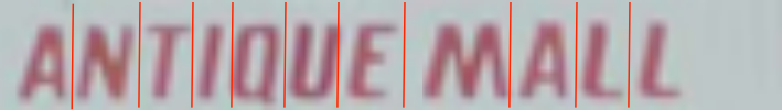
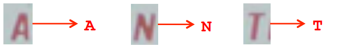
photo OCR流水线如下所示。

Sliding windows

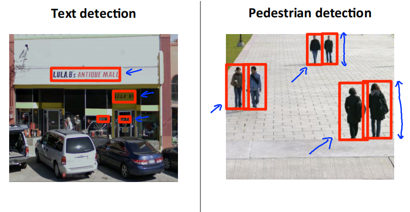
文字识别在计算机视觉中是一个比较难的问题，因为文字区域对应的矩形有着不同的长宽比。我们先从简单的行人检测开始。行人检测要识别的对象具有相似的长宽比，所以仅用一个固定长宽比的而矩形就可以了

supervised learning for pedestrian detection

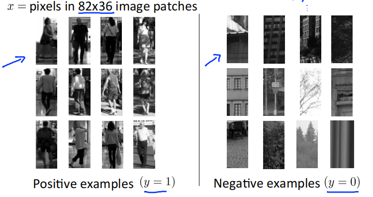
定义矩形大小为82*36。从数据集中收集一些正样本和负样本。通过这些样本训练一个分类器，用来判断图中是否包含行人。

Sliding window detection

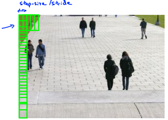
用一个固定大小的矩阵按照从上到下，从左到右的顺序，依次获取矩形中的图像，将其传递给分类器判断图像是否存在行人。矩形每次移动的距离称为步长，1px的步长效果最好，但是计算量较大，一般取4px，8px等。矩形的大小可以自定义，从而获取大小不同的图像。获取的图像通过一定的缩放之后，达到82*36的大小，再放入分类器中进行识别。

Text detection

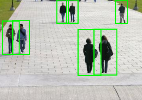
文字识别也训练出一个分类器来，判断图像中是否存在文字。

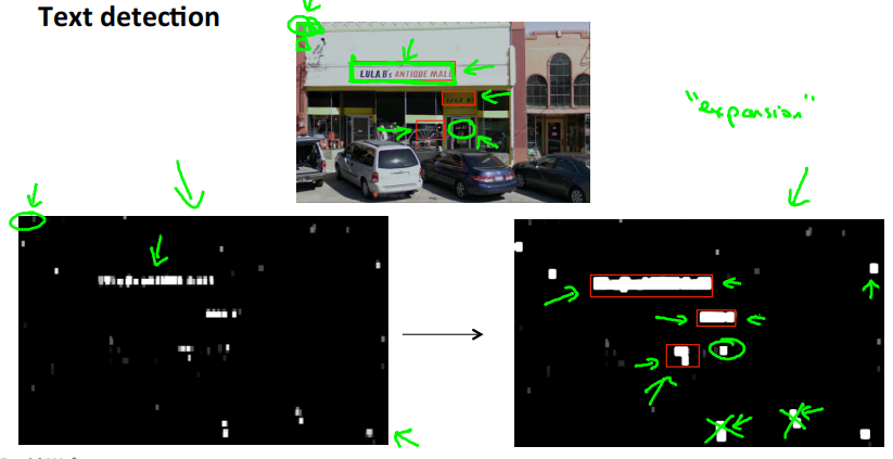
使用滑动窗口，识别出图中存在文字的地方，识别结果如左下图所示。白色的部分表示文本检测系统发现了文本；黑色部分表示没有发现文字； 深浅不同的灰色表示分类器认为该处有文字的概率。

将分类器的结果应用到一个叫放大算子的东西上。它把每个白色区域都进行扩大。具体地说，如果左边图片中，某个像素的一定范围内存在白色像素，那么就在右图中把它变成白色。即原来白色的区域向外扩大一部分。

完成之后，在右图白色区域周围绘制边框。同时也可以过滤一些比例很奇怪的矩形，因为文本周围的框，宽度应该大于高度。

处理完成之后，把这些区域剪切出来，进入流水线的下一个阶段

1D sliding window for character segmentation

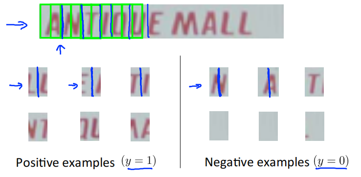
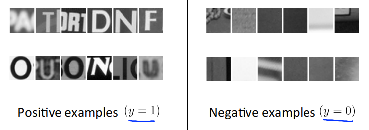
再次使用监督学习，用一些正样本和负样本，训练出一个分类器，判断是否存在字符分割的地方。

使用滑动窗口，从左到右移动，判断窗口内的图像是否存在字符分割的地方，然后对图像进行分割。

Getting lots of data : Artificial data synthesis

一个最可靠的得到高性能机器学习系统的方法是使用一个低偏差机器学习算法，并且使用庞大的训练集去训练它。

为了获取更多的数据可以使用人工数据合成，但它并不适用于所有问题，而且将其运用于特定问题时，经常需要思考改进并且深入了解它。

人工数据合成主要有两种形式：一种是自己创造数据，即从零开始创造新数据；第二种是我们已经有小的标签训练集，然后以某种方式扩充训练集。

Artificial data synthesis for photo OCR

用不同的字体生成字符，然后将其粘贴到任意不同的背景。可以应用一点模糊算子或者仿射变换（等分、缩放、旋转等操作）

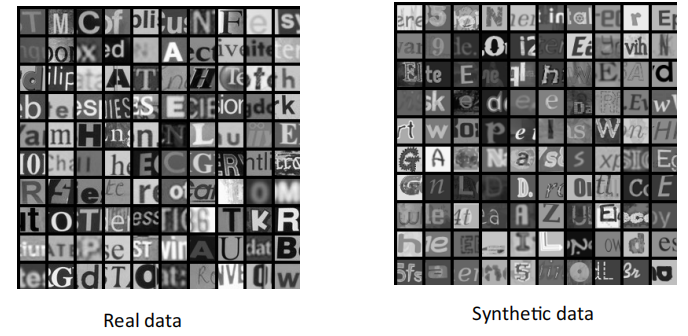
新生成的数据与原来的真实数据非常相似，那么使用合成的数据，就可以为训练提供无限的数据样本。如果合成的数据做的不好，那训练的效果也会不好。

Synthesizing data by introducing distortions

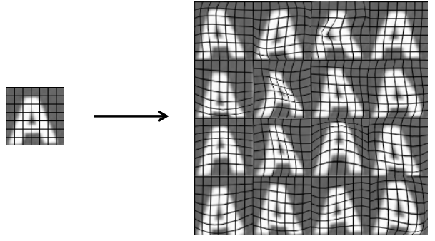
对图片进行人工拉伸、人工扭曲从而获得更大的数据集。

对于一些音频片段，想从中学习、识别语音片段中出现的单词。假定有一个带标签的训练样本，可以引入额外的语音失真到数据集中。比如增加背景音模拟在街道上，在工厂，手机信号不好。

Distortion introduced should be representation of the type of noise/distortion in the test set。

在引入失真合成数据时，引入的失真应该具有代表性，这些噪音和扭曲是有可能出现在测试集中的。

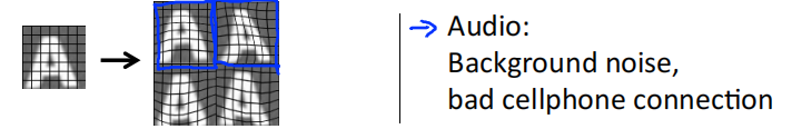
Usually does not help to add purely random/meaningless noise to your data

如果只是将随机的无意义的噪音加入到数据中，则并没有多大帮助。下图中，右边4张图中的每个像素随机加入了一些高斯噪音，即改变每个像素的亮度，这样的噪音是完全没有意义的。除非你觉得可能在测试集中看到这种像素级别的噪音，不然很可能就是无用的。

Discussion on getting more data

1. Make sure you have a low bias classifier before expending the effort.(Plot learning curves).E.g. keep increasing the number of features/number of hidden units in neural network until you have a low bias classifier.
2. "How much work would it be to get 10x as much data as we currently have"
   • Artifical data synthesis
   • Collect/label it yourself
   • "Crowd source"(E.g. Amazon Mechanical Turk)

Ceiling analysis:What part of the pipeline to work on next

Estimating the error due to each component (ceiling analysis)

What part of the pipeline should you spend the most time trying to improve?

在测试集上，一开始整个系统的正确率在72%。

文本检测模块：

模拟文本检测模块是100%的正确率，观察其对整个系统的影响。对于测试集，对于每一个测试集样本都提供一个正确的文本检测结果，即遍历每个测试集样本，人为地告诉算法每个测试样本中文本的位置。或者说我们模拟100%正确地检测出图片中的文本信息，然后将它传递给下一个模块。然后继续运行完后两个模块，测量整个系统的准确率。假设正确的文本检测模块将系统的准确率提高到了89%。

字符分割模块：

模拟字符分割模块是100%的正确率，观察其对整个系统的影响。对于得到的准确的文本检测结果，人为地把文本分割成单个字符，得到100%正确的字符分割结果，然后把它传递给下一个模块。然后继续运行下一个模块，测量整个系统的准确率。假设正确的字符分割模块将系统的准确率提高到了90%。

字符识别模块：

同样是人工给出这一模块的正确标签，理所当然得到100%的正确率。

进行上限分析的好处是我们知道了如果对每一个模块进行完善，它们各自的上升空间是多少。 比如完美的文本检测模块提高了17%的正确率，所以值得花费大量精力去提升；完美的字符分割模块提升了1%的正确率，不值得花费大力气去完善。

Component	Accuracy
Overall system	72%
Text detection	89%
Character segmentation	90%
Character recognition	100%

another ceiling analysis example

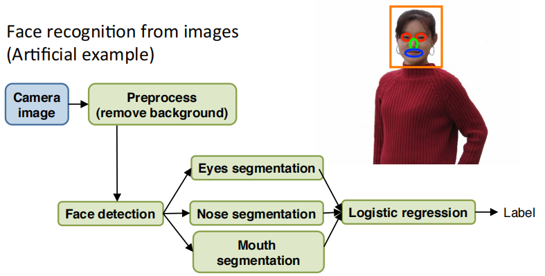
假如用图片做人脸识别。这是一个偏人工智能的例子，当然这并不是现实中的人脸识别技术。

首先是图像预处理，去除背景。

然后是用滑动窗口进行人脸检测。

然后分割出眼睛，分割出鼻子，分割出嘴巴

把所有特征输入给某个逻辑回归分类器

最终给出标签。

Component	Accuracy
Overall system	85%
Preprocess (remove background)	85.1%
Face detection	91%
Eye segmentation	95%
Nose segmentation	96%
Mouth segmentation	97%
logistic regression	100%

不要相信直觉，如果要解决某个机器学习问题，最好能把问题分成多个模块，然后做一下上限分析，这通常会给你更好的方法，来决定往哪个方向努力，该提高哪个模块的效果