Lecture15 Anomaly detection
Lecture 15 Anomaly detection
problem motivation
Gaussian distribution
Algorithm
Density estimation
Training set : \({x^{(1)},x^{(2)},\dots,x^{(m)}}\)
Each example is \(x \in \mathbb{R}^n\)
Anomaly detection algorithm
-
Choose features \(x_i\) that you think might be indicative of anomalous example
-
Fit parameters \(u_1,u_2,\dots,u_n,\sigma_1^2,\sigma_2^2,\dots,\sigma_n^2\)
\(u_j=\frac{1}{m}\sum_{i=1}^mx_j^{(i)}\)
\(\sigma_j^2=\frac{1}{m}\sum_{i=1}^m(x_j^{(i)}-u_j)^2\)
-
Given new example \(x\),compute \(p(x)\)
\[p(x)=\prod_{j=1}^np(x_j,u_j,\sigma_j^2)=\prod_{j=1}^n\frac{1}{\sqrt{2\pi}\sigma_j}exp(-\frac{(x_j-u_j)^2}{2\sigma^2_j}) \]Anomaly if \(p(x)<\varepsilon\)
Anomaly detection example
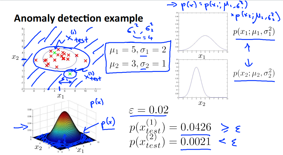
\(x_1\sim N(5,4)\),\(x_2\sim N(3,1)\)
对于测试样本\(x_{test}^{(1)}\),其坐标为\((a,b)\),计算其落在横坐标\(a\)上的概率\(p(a,u_1,\sigma_1^2)\),落在纵坐标\(b\)上的概率\(p(b,u_2,\sigma_2^2)\)。\(p(x) = p(a,u_1,\sigma_1^2)p(b,u_2,\sigma_2^2)\)就是测试样本\(x_{test}^{(1)}\)落在平面上点\((a,b)\)的概率。因为\(p(x_{test}^{(1)})=0.0426 \geq \varepsilon\) 所以判定其为正常样本。
同理,\(p(x_{test}^{(2)})=0.0021 \leq \varepsilon\) 所以判定其为异常样本
Developing and evaluating an anomaly detection system
The inportance of real-number evaluation
When developing a learning algorithm (choosing features,etc.),making decisions is much easier if we have a way of evaluating our learning algorithm
Assume we have some labeld data,of anomalous and non-anomalous example(y = 0 if normal,y = 1 if anomalous)
Training set:\(x^{(1)},x^{(2)},\dots,x^{(m)}\) (assume normal examples/not anomalous).把训练集是正常样本的集合,即使溜进了一些异常样本。
Cross validation set: \((x_{cv}^{(1)},y_{cv}^{(1)}),\dots,(x_{cv}^{(m_{cv})},y_{cv}^{(m_{cv})})\)
Test set : \({(x_{test}^{(1)},y_{test}^{(1)}),\dots,(x_{test}^{(m_{test})},y_{test}^{(m_{test})})}\)
验证集和测试集都包含一些异常样本
Aircraft engines motivating example
10000 good (normal) engines
20 flawd engines (anomalous)
Training set : 6000 good engines (y = 0)
CV : 2000 good engines (y = 0),10 anomalous (y = 1)
Test : 2000 good engines (y = 0),10 anomalous (y = 1)
Alternative : (不推荐)
Training set : 6000 good engines (y = 0)
CV : 4000 good engines (y = 0),10 anomalous (y = 1)
Test : 4000 good engines (y = 0),10 anomalous (y = 1)
验证集和测试集应当是两个完全不同的数据集。
Algorithm evaluation
Fit model \(p(x)\) on training set \(\{x^{(1)},\dots,x^{(m)}\}\)
On a cross validation/test example \(x\),predict
possible evaluation metrics:
- True positive,false positive,false negative,true negative
- Precision/Recall
- \(F_1\)-score
Can also use cross validation set to choose parameter \(\varepsilon\)
尝试许多不同的 \(\varepsilon\),找到使得\(F_1\)-score最大的\(\varepsilon\)
Anomaly detection vs. supervised learning
| Anomaly detection | Supervised learning |
|---|---|
| vary small number of positive example (y = 1).(0-20 is common) Large number of negative (y = 0) examples | Laege number of positive and negative examples |
| Many different “types" of anomalies.Hard for any algorithm to learn from positive examples what the anomalies look like ; future anomalies may look nothing like any of the anomalous examples we've seen so far | Ecough positive examples for algorithm to get a sense of what positive examples are like,future positive examples likely to be similar to ones in training set |
异常检测适用于正样本少,负样本多的情况。监督学习适用于正负样本都多的情况。
异常有很多种,异常样本较少,很难从正样本中学习异常。而且将来出现的异常很可能会与已有的截然不同。适用于异常检测。
监督学习拥有足够多的正样本去学习异常,而且将来出现的异常与当前训练集中的正样本相似。适用于监督学习。
关键是正样本的数量。
| Anomaly detection | Supervised learning |
|---|---|
| Frad detection | Email spam classification |
| Manufacturing (e.g. aircraft engines) | Wheater prediction |
| Monitoring machines in a data center | Cancer classification |
Choosing what features to use
Non-gaussian features
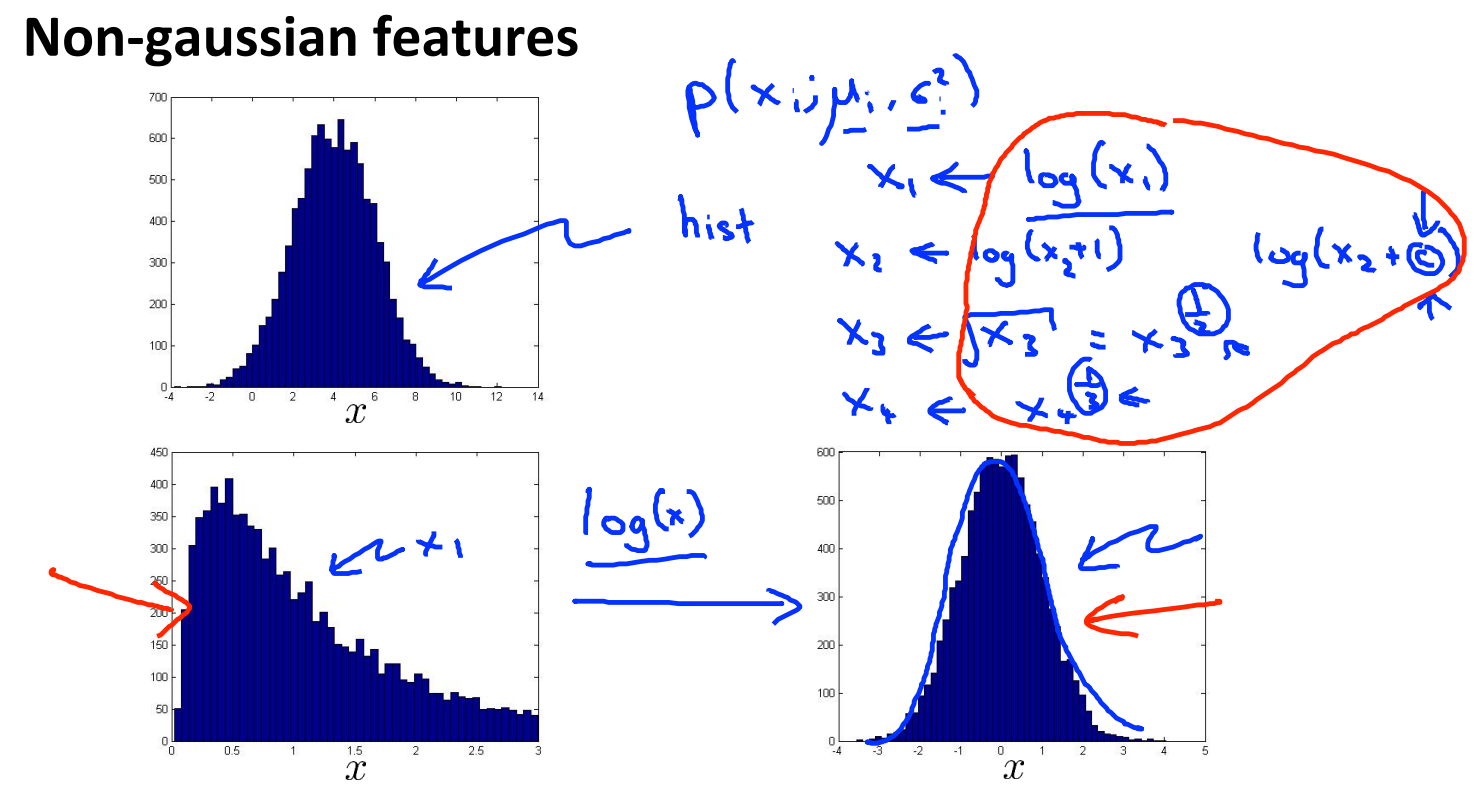
对于不符合高斯分布的数据,通过对数据进行一些转换,使得它看上去更接近高斯分布。虽然不进行转换算法也可以运行,但转换之后,算法可以运行的更好。
通常的转换方式有
Error analysis for anomaly detection
Want \(p(x)\) large for normal examples \(x\)
\(p(x)\) small for anomalous examples \(x\)
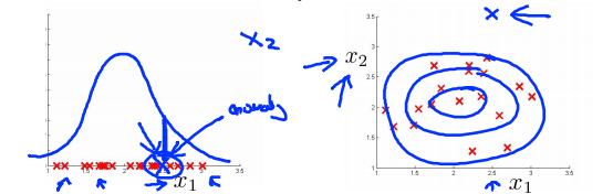
Most common problem : \(p(x)\) is comparable (say,both large) for normal and anomalous examples.
发现一个新的特征\(x_2\),他能够将异常样本和正常样本区分开来。
Monitoring computers in a data center
Choose features that might take on unusually large or small values in the event of an anomaly
\(x_1\)=memory use of computer
\(x_2\)=number of disk accesses/sec
\(x_3\)=CPU load
\(x_4\)=network traffic
\(x_5\)=CPU load / network traffic
\(x_6\)=(CPu load)^2 / network traffic
Multivariate Gaussian distribution
Motivating example:Monitoring machines in a data center
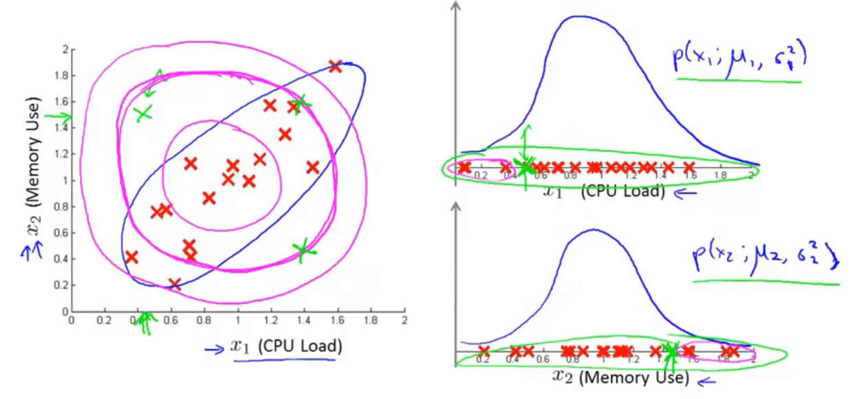
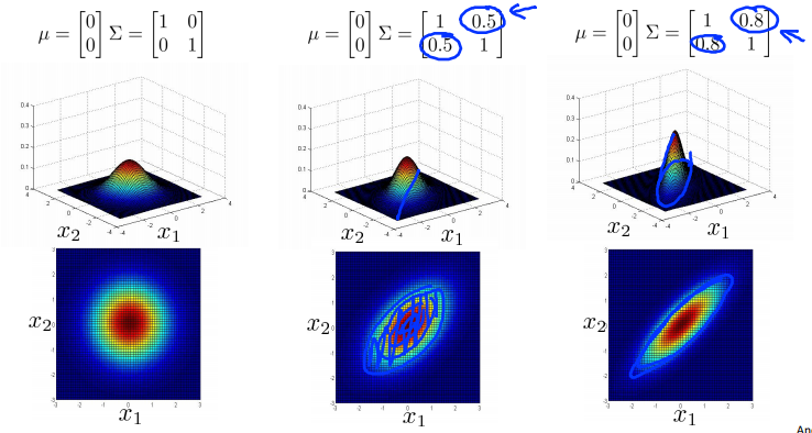
对于绿色样本\(x^{(1)}(0.5,1.5)\),CPU负载很低,但内存使用量很高,是一个异常样本。如果认为两个变量线性无关,计算结果\(p(x^{(1)})=p(x_1^{(1)},u_1,\sigma_1^2)p(x_2^{(1)},u_2,\sigma_2^2)\)并不低,所以可能不会被归类为异常样本。紫红色的等高线图表示其概率在平面上的分布。但是CPU负载和内存使用量之间存在线性关系。其概率分布是椭圆形的。
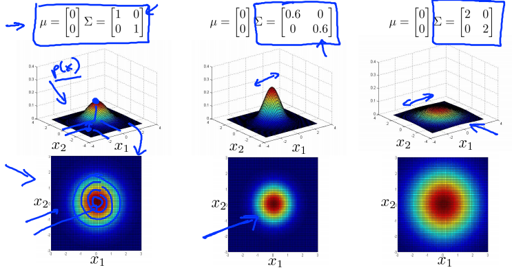
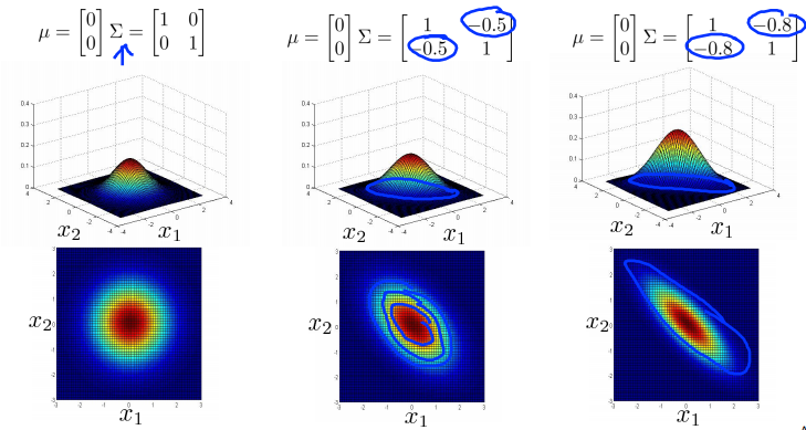
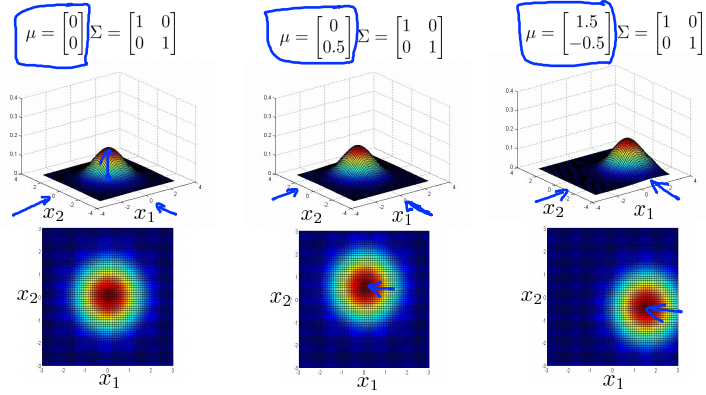
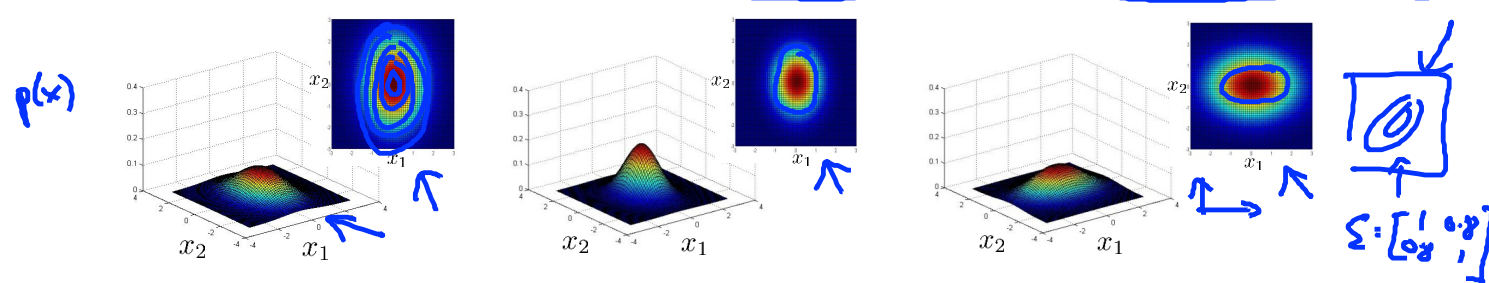
Multivariate Gaussian (Normal) distribution
\(x\in\mathbb{R}^n\). Don't model \(p(x_1),p(x_2),\dots\),etc. separately.
Model \(p(x)\) all in one go.
Parameters : \(u \in \mathbb{R}^n\),\(\Sigma \in \mathbb{R}^{n\times n}\)(covariance matrix)
Parameter fitting:
Given training set \(\{x^{(1)},x^{(2)},\dots,x^{(m)}\}\)
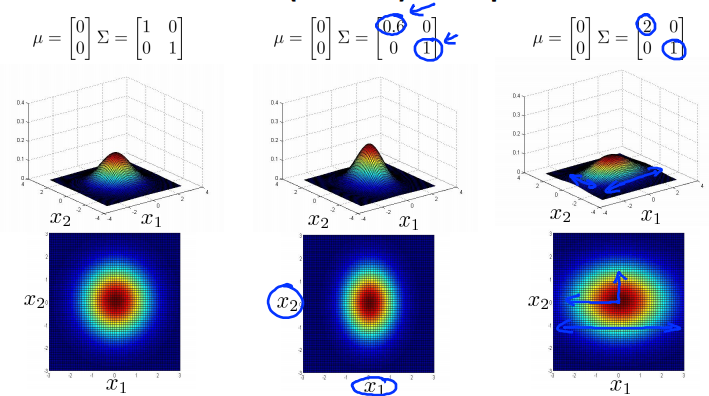
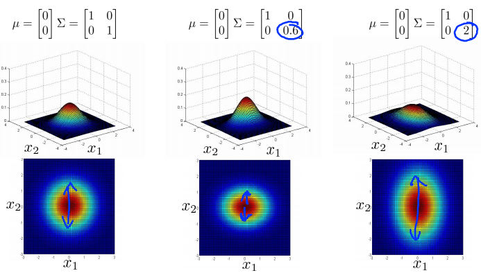
Multivariance Gaussian (Normal) examples
Anomaly detection using the multivariance Gaussian distribution
Relationship to origin model
Original model : \(p(x) = p(x_1,u_1,\sigma_1^2)p(x_2,u_2,\sigma_2^2)\dots p(x_n,u_n,\sigma_n^2)\)
Corresponds to multivariate Gaussian
Where \(\Sigma = \left[\begin{matrix}\sigma^2_1&0&\cdots&0\\0&\sigma^2_2&\cdots&0\\\vdots&\vdots&\ddots&\vdots\\0&0&\cdots&\sigma^2_n\end{matrix}\right]\)
原模型的等高线图总是轴对齐的 (axis-aligned)。(变量之间线性无关。)
| Original model | Multivariate Gaussian |
|---|---|
| Manually create features to capture anomalies where \(x_1,x_2\) take unusual combinations of values.e.g.\(x_3=\frac{x_1}{x_2}=\frac{CPU\ load}{memory}\) | Automaticlly capture correlations between features |
| Computationally cheaper(alternatively,scales better to large) | Computationally more expensive |
| OK even if \(m\) (training set size) is small | Must have \(m>n\) or else \(\Sigma\) is non-invertible (\(m \geq 10n\)) |
本文来自博客园,作者:Un-Defined,转载请保留本文署名Un-Defined,并在文章顶部注明原文链接:https://www.cnblogs.com/EIPsilly/p/15711247.html

 浙公网安备 33010602011771号