吴恩达机器学习第二章作业：线性回归，TASK1 逻辑回归（python实现）

TASK 1任务要求：实现预测学生被录取的几率。

数据集：现在有100名学生的数据集，col1 是考试一的分数，col2 是考试二的分数，col3 是该学生是否被录取

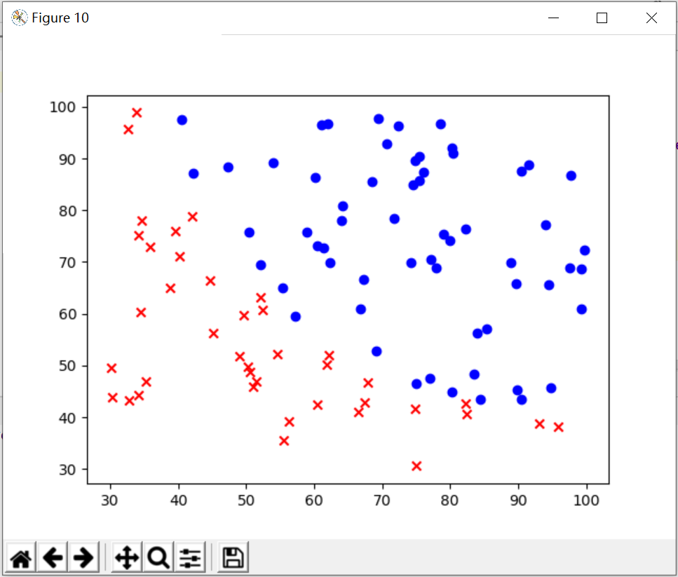
1、实现数据的可视化

data = pd.read_csv('D:\python学习\吴恩达机器学习\ex2data1.txt',header=None,names=['subject1','subject2','admit'])
X = data.iloc[:,0:-1] # DataFrame用iloc取列
y = data.iloc[:,-1]
X = X.values
y = y.values
plt.figure(10)
ax = plt.subplot()
ax.scatter(X[y==1,0],X[y==1,1],marker='o',c='b')
ax.scatter(X[y==0,0],X[y==0,1],marker='x',c='r')
plt.show()

这个上一个稿件也说明了怎么样使数据可视化，现在不再赘述。只是倒数第二行和倒数第三行的散点图的绘制要学习一下！

绘制效果如图：

2、实现sigmoid函数（也就是s型函数）

def sigmoid(z):
    return 1 / (1 + np.exp(- z))

3、计算初始时的cost的值是多少

再定义一个函数：

def computecost(theta, x, y):
    first = (-y) * np.log(sigmoid(x @ theta))     #cost函数前面的项  @是矩阵乘法
    second = (1 - y)*np.log(1 - sigmoid(x @ theta))   #cost函数后面的项
    return np.mean(first - second)  # 求均值

cost =  0.6931471805599453

4、计算梯度：（因为在这个例子里面梯度不能和优化一起跟新theta，所以只能先算梯度，后算优化）

def gradient(theta, x, y):
    return (x.T @ (sigmoid(x @ theta) - y))/len(x)

5、进行优化，我们优化不必像前一个例子一样自己手动计算theta之后跟新的值，我们可以借助优化函数：

result = opt.fmin_tnc(func=computecost, x0=theta, fprime=gradient, args=(x, y))   #func:优化的目标函数  fprime：梯度函数 args：数据 x0 初值

最后得到的result时一个array，我们要将他变为向量；采用final_theta = result[0]，来使array变成向量

最后得到的向量为：

final_theta = [-25.16131846   0.20623159   0.20147148]

代表了theta0（偏置），theta1（x1的权重），theta2（x2的权重）

6、绘制决策边界：

x1 = np.arange(130, step=0.1)
x2 = -(final_theta[0]+final_theta[1]*x1)/final_theta[2]


plt.figure(10)
ax = plt.subplot()
ax.scatter(x[y==1,0],x[y==1,1], color='blue', marker = 'o')
ax.scatter(x[y==0,0],x[y==0,1], color='red', marker='x')
ax.plot(x1, x2)
ax.set_xlabel('x1')
ax.set_ylabel('x2')
ax.set_title('Decision Boundary')
plt.show()

先规定x1的范围，然后再通过公式：theta0 + theta1*x1 + theta2*x2 = 0来解出 x2 = -（theta0+theta1*x1）/ theta2

然后再画出决策边界，如下图：

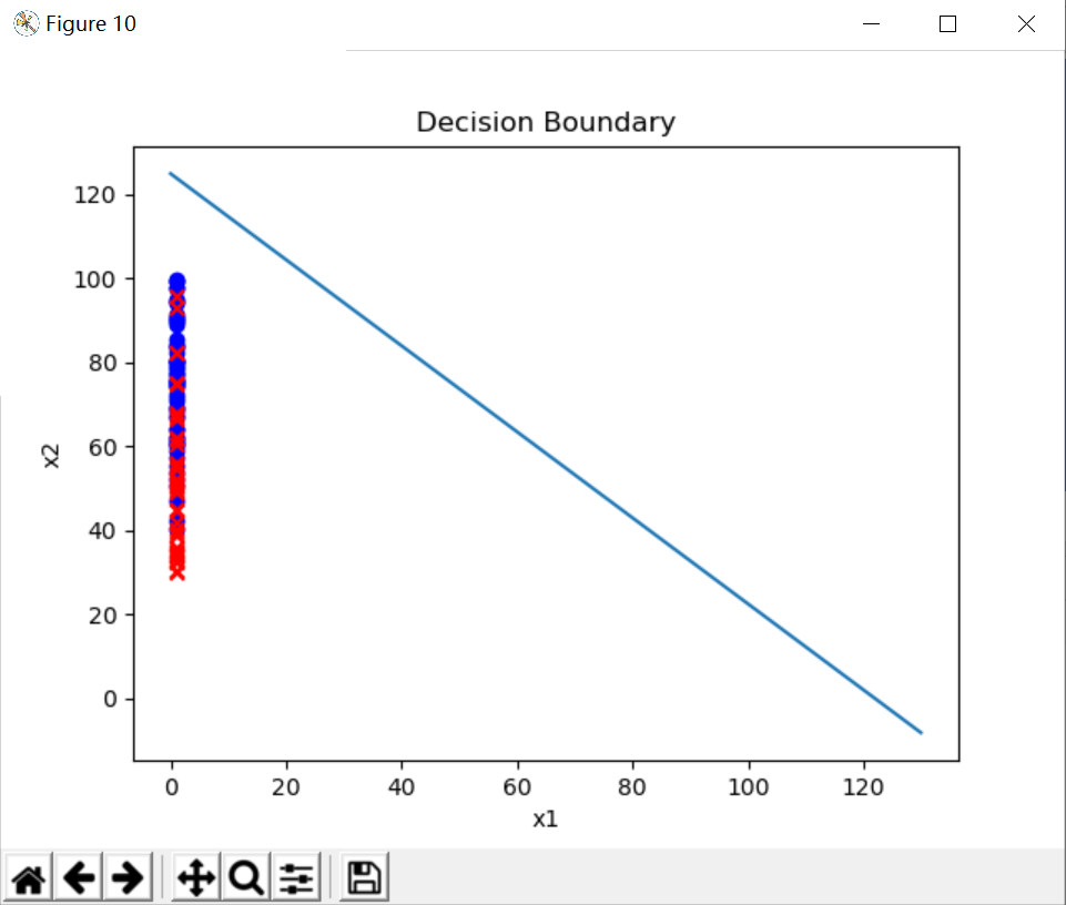
最后的散点图没有能绘制好，我尝试的所有办法都不能让exam1score的分数从 x1 = 1 的这个线移开，但是决策边界已经写好了，TASK1也就完成了。

最后附上所有的代码：

import numpy as np
import pandas as pd
import matplotlib.pyplot as plt
import scipy.optimize as opt
data = pd.read_csv('D:\python学习\吴恩达机器学习\ex2data1.txt',header=None,names=['subject1','subject2','admit'])
x = data.iloc[:,0:-1] # DataFrame用iloc取列
y = data.iloc[:,-1]
x = x.values
y = y.values
theta = np.zeros(x.shape[1])  #设定theta初始值为0
plt.figure(10)
ax = plt.subplot()
ax.scatter(x[y==1,0],x[y==1,1],marker='o',c='b')
ax.scatter(x[y==0,0],x[y==0,1],marker='x',c='r')
plt.show()


def sigmoid(z):
    return 1 / (1 + np.exp(- z))

def computecost(theta, x, y):
    first = (-y) * np.log(sigmoid(x @ theta))     #cost函数前面的项  @是矩阵乘法
    second = (1 - y)*np.log(1 - sigmoid(x @ theta))   #cost函数后面的项
    return np.mean(first - second)  # 求均值
print(computecost(x,y,theta))


def gradient(theta, x, y):
    return (x.T @ (sigmoid(x @ theta) - y))/len(x)
data = pd.read_csv('D:\python学习\吴恩达机器学习\ex2data1.txt', names=['exam1', 'exam2', 'admitted'])# 读入数据 标记列名

#接下来预测学生是否被录取，写决策边界
def predict(theta,x):
    h_theta = sigmoid(x @ theta)
    return [1 if x>=0.5 else 0 for x in h_theta]

data.insert(0, 'Ones', 1)         # 在data中加一列x0
x = data.iloc[:,0:-1] # DataFrame用iloc取列
y = data.iloc[:,-1]
x = x.values
y = y.values

theta = np.zeros(x.shape[1])  #设定theta初始值为0
result = opt.fmin_tnc(func=computecost, x0=theta, fprime=gradient, args=(x, y))   #func:优化的目标函数  fprime：梯度函数 args：数据 x0 初值

final_theta = result[0]
print(final_theta)

#predictions = predict(final_theta,x)
#correct = [1 if a==b else 0 for (a,b) in zip (predictions,y)]
#accuracy = sum(correct)/len(x)
#print(accuracy)

#绘制决策边界

x1 = np.arange(130, step=0.1)
x2 = -(final_theta[0]+final_theta[1]*x1)/final_theta[2]


plt.figure(10)
ax = plt.subplot()
ax.scatter(x[y==1,0],x[y==1,1], color='blue', marker = 'o')
ax.scatter(x[y==0,0],x[y==0,1], color='red', marker='x')
ax.plot(x1, x2)
ax.set_xlabel('x1')
ax.set_ylabel('x2')
ax.set_title('Decision Boundary')
plt.show()