吴恩达机器学习第一章作业：线性回归，TASK2 多变量线性回归（python实现）

TASK2 多变量线性回归

由于是多变量线性回归，所以数据不一定可视化，就比如这个例子：

第一列是房屋的面积x1，第二列是房屋的房间数量x2，第三列是房屋的售价y，由公式可以这么写：

x1————x2————（f）————y

也就是x1和x2都对y有影响，道理和单变量线性回归类似：

1、先进行多变量的归一化，让数据显得不是那么庞大：

path = 'D:\python学习\吴恩达机器学习\ex1data2.txt'
data = pd.read_csv(path,names = ['feets','bedrooms','price'])
data = (data-data.mean())/data.std()##已经处理完数据，进行了归一化操作了

这里解释一下data.mean()是data的平均数，data.std()是data的方差，归一化的公式为：

x.归一化 =( x-x.mean )/x.std

2、照例写出cost的函数

def computecost(x,y,theta):
    h_x = x*theta.T
    temp = np.power((h_x-y),2)
    J_theta = np.sum(temp)/(2*len(x))
    return J_theta

3、写出梯度下降的函数

def gradientdiscent(x,y,theta,epoch,alpha):
    temp = np.matrix(np.zeros(theta.shape))
    cost = np.zeros(epoch)
    for i in range(epoch):
        temp = theta-(alpha/len(x))*(x*theta.T-y).T*x
        theta = temp
        cost[i] = computecost(x,y,theta)
    return theta,cost

以上两个函数和单变量线性回归基本上一样

4、计算一下theta未跟新时的cost值

data.insert(0,'ones',1)
col = data.shape[1]
x = data.iloc[:,0:col-1]
y = data.iloc[:,col-1:col]
x = np.matrix(x.values)
y = np.matrix(y.values)
theta = np.matrix([0,0,0])

计算出来cost = 0.48936

已经很小了，但是这是归一化之后的cost，原来的cost应该还是非常大，所以要进行梯度下降来跟新theta，使cost变小

5、跟新theta

epoch = 1000
alpha = 0.01
theta,cost = gradientdiscent(x,y,theta,epoch,alpha)##算出来theta和cost了

6、绘制cost曲线图

fig,m = plt.subplots(figsize =(6,6) )
m.plot(np.arange(epoch),cost,'blue')
m.set_xlabel('iters')
m.set_ylabel('cost')
plt.show()

cost的曲线图如下图所示：

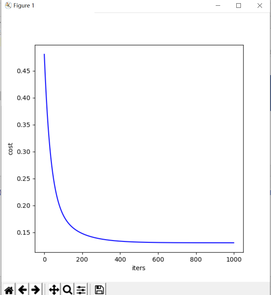
可以看出，跟新到300次之后cost已经基本稳定在0.13附近，还是比较小的。

 

 

 

完整代码如下：

import numpy as np
import pandas as pd
import matplotlib.pyplot as plt
path = 'D:\python学习\吴恩达机器学习\ex1data2.txt'
data = pd.read_csv(path,names = ['feets','bedrooms','price'])
data = (data-data.mean())/data.std()##已经处理完数据，进行了归一化操作了
#写代价函数了
def computecost(x,y,theta):
    h_x = x*theta.T
    temp = np.power((h_x-y),2)
    J_theta = np.sum(temp)/(2*len(x))
    return J_theta

data.insert(0,'ones',1)
col = data.shape[1]
x = data.iloc[:,0:col-1]
y = data.iloc[:,col-1:col]
x = np.matrix(x.values)
y = np.matrix(y.values)
theta = np.matrix([0,0,0])
##算出来costfunction为0.4893617021276595

#接下来算gradientdiscent了，来跟新theta
def gradientdiscent(x,y,theta,epoch,alpha):
    temp = np.matrix(np.zeros(theta.shape))
    cost = np.zeros(epoch)
    for i in range(epoch):
        temp = theta-(alpha/len(x))*(x*theta.T-y).T*x
        theta = temp
        cost[i] = computecost(x,y,theta)
    return theta,cost
epoch = 1000
alpha = 0.01
theta,cost = gradientdiscent(x,y,theta,epoch,alpha)##算出来theta和cost了
##下面开始绘制cost的下降梯度

fig,m = plt.subplots(figsize =(6,6) )
m.plot(np.arange(epoch),cost,'blue')
m.set_xlabel('iters')
m.set_ylabel('cost')
plt.show()