吴恩达机器学习第一章作业：线性回归，TASK1单变量线性回归（python实现）

TASK1：单变量线性回归

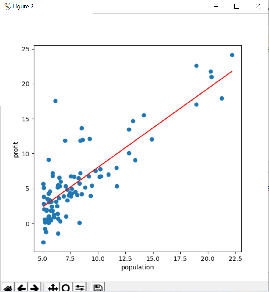
          data1表示的是人口的利润的关系，第一列表示的是人口（population），第二列表示的是利润（profit）。我们要根据人口来预测利润，所以确定好了人口（population)是x，利润（profit）是y。类似于:

x——（f)  ——y

这种映射。

1、ploting the data

这个就不用多说了 ，直接有代码：

path = 'D:\python学习\吴恩达机器学习\ex1data1.txt'
data = pd.read_csv(path,names = ['population','profit'])
data.plot (kind='scatter',color = 'red',x = 'population',y = 'profit')#这里解释一下kind = ‘scatter’就是散点图的意思
plt.show()

实现的效果如图：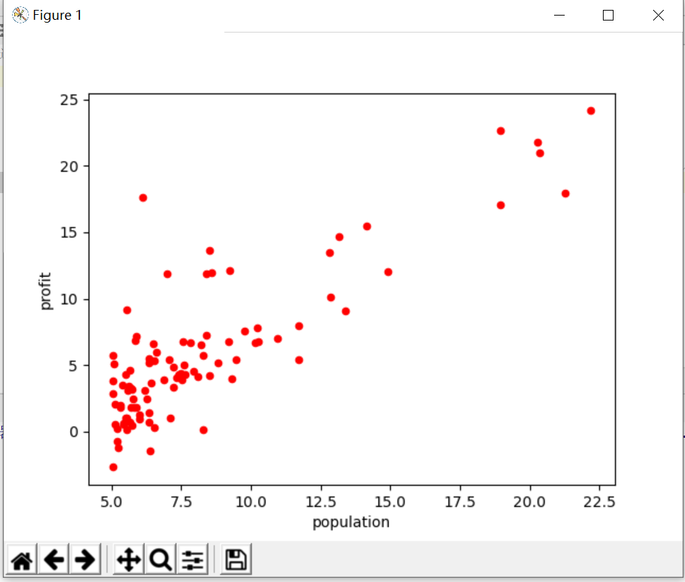

 

2、gradient descent 梯度下降

这里是实现优化的第一个难点，运用梯度下降来跟新theta

公式就如上图所写，接下来就是要用代码实现这个公式。

定义函数computecost 来计算cost的值

def computecost(x,y,theta):
    h_x = x*theta.T #x经过处理之后是97行2列的向量，theta是x的权重，根据x的大小在变化
    temp = np.power((h_x-y),2)
    J_theta = np.sum(temp)/(2*len(x))
    return J_theta
#不能直接计算J_theta，要用temp做中间变量，这一点老师在课中讲过了，现在不赘述

定义函数gradientdiscent，跟新theta的值（discent 定义函数的时候打错了，干脆将错就错）

def gradientdiscent(x, y, theta ,epoch, alpha):
    temp = np.matrix(np.zeros(theta.shape))#临时变量，盛放之后的theta用的
    cost = np.zeros(epoch)#为下面的cost【i】做准备用的
    for i in range (epoch):
        temp = theta-(alpha/len(x))*(x*theta.T-y).T*x
        theta = temp
        cost[i] = computecost(x,y,theta)

    return theta,cost
#epoch是跟新的此数，每一次跟新都会遍历整个x的值，然后跟新一次theta

现在就知道了最好的theta 和最小的cost了。

3、算一下初始的cost有多少：（也就是theta=【0，0】时的cost值）

data.insert(0,'ones',1)
col = data.shape[1]#列数，同理data.shape[0]为行数
x = data.iloc[:,0:col-1]
y = data.iloc[:,col-1:col]
x = np.matrix(x.values)#这个操作是为了把x作为97行2列的大矩阵，拆分成97个1行2列的小矩阵，便于计算
y = np.matrix(y.values)#同理
theta = np.matrix([0,0])
print(computecost(x,y,theta))

计算出来的cost = 32.072733877455676

4、计算一下跟新theta之后的cost的值

alpha = 0.01
epoch = 1000
theta,cost = gradientdiscent(x,y,theta,epoch,alpha)
print(computecost(x,y,theta))

学习率alpha = 0.01

跟新次数epoch先设定成1000次，然后会酌情增加或者减少此数，这些都是根据cost大小来定的。

输出的最小cost = 4.515955503078914，应该是最小的cost值了，我们可以绘制predicted曲线了

5、绘制预测曲线

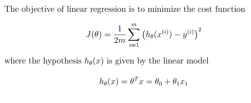
跟新之后的theta是一个一行两列的向量，theta的第一个元素是偏置b，theta的第二个元素是斜率k，根据这个我们可以得出预测曲线可以这么写：

y = theta【0，0】+theta【0，1】*x

然后把图像表示出来就行了：

x= np.linspace(data.population.min(),data.population.max(),10)   #先定下来x轴的坐标，x轴坐标定下来了y轴坐标也就自动定下来了
function = theta[0,0]+theta[0,1]*x
fig,m =plt.subplots(figsize = (6,6))
m.plot(x,function,color='red',label = 'prediction')  ##这是给图像设定一些参数
m.scatter(data['population'], data['profit'], label='Traning Data')
m.set_xlabel('population')
m.set_ylabel('profit')
plt.show()

得到的图线如下图;

 

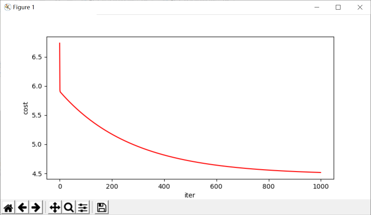
6、绘制cost曲线，看跟新多少次之后cost变得最小了

fig,m = plt.subplots(figsize = (8,4))
m.plot(np.arange(epoch),cost,'r')##这一步是关键，内容变成了cost
m.set_xlabel('iter')
m.set_ylabel('cost')
plt.show()

结果如下图所示

 

TASK1结束

整段代码如下：

import numpy as np
import pandas as pd
import matplotlib.pyplot as plt
path = 'D:\python学习\吴恩达机器学习\ex1data1.txt'
data = pd.read_csv(path,names = ['population','profit'])
data.plot (kind='scatter',color = 'red',x = 'population',y = 'profit')
#plt.show()

def computecost(x,y,theta):
    h_x = x*theta.T
    temp = np.power((h_x-y),2)
    J_theta = np.sum(temp)/(2*len(x))
    return J_theta
data.insert(0,'ones',1)
col = data.shape[1]#列数
x = data.iloc[:,0:col-1]
y = data.iloc[:,col-1:col]
x = np.matrix(x.values)
y = np.matrix(y.values)
theta = np.matrix([0,0])
print(computecost(x,y,theta))
##上面都是完成了初始设置，得到初始的costfunction的结果是32左右，下面进行梯度下降

def gradientdiscent(x, y, theta ,epoch, alpha):
    temp = np.matrix(np.zeros(theta.shape))
    cost = np.zeros(epoch)
    for i in range (epoch):
        temp = theta-(alpha/len(x))*(x*theta.T-y).T*x
        theta = temp
        cost[i] = computecost(x,y,theta)

    return theta,cost
alpha = 0.01
epoch = 1000
theta,cost = gradientdiscent(x,y,theta,epoch,alpha)
print(computecost(x,y,theta))
##输出的costfunction为4.51，差不多是最小的cost值了
##接下来就是绘制拟合图线了
##theta[0,0]表示的是theta的第零行，第零列，为一个数字

x= np.linspace(data.population.min(),data.population.max(),10)
function = theta[0,0]+theta[0,1]*x
fig,m =plt.subplots(figsize = (6,6))
m.plot(x,function,color='red',label = 'prediction')
m.scatter(data['population'], data['profit'], label='Traning Data')
m.set_xlabel('population')
m.set_ylabel('profit')
plt.show()


##绘制epoch和cost关系
fig,m = plt.subplots(figsize = (8,4))
m.plot(np.arange(epoch),cost,'r')
m.set_xlabel('iter')
m.set_ylabel('cost')
plt.show()