小匠第一周期打卡笔记-Task01
一、线性回归
知识点记录
线性回归输出是一个连续值,因此适用于回归问题。如预测房屋价格、气温、销售额等连续值的问题。是单层神经网络。
线性判别模型
判别模型
性质:建模预测变量和观测变量之间的关系,亦称作条件模型
分类:确定性判别模型:y=fθ(x)
概率判别模型:pθ(y|x)
线性判别模型(linear regression)
y=fθ(x)= θo +【(d,i=1),加和】θjxj = θTx ,x= (x1,x2,x3,...,xd)
学习目标:
使预测值和真实值的距离越近越好, min 1((【N,i=1】)加和)&(yi,fθ(xi)))/N
损失函数:&(yi,fθ(xi))测量预测值与真实值之间的误差,越小越好(方差最小),
具体损失函数的定义依赖于具体数据和任务
最广泛使用的损失的回归函数:平方误差(squared loss),&(yi,fθ(xi)) = 1(yi-fθ(xi))*(yi-fθ(xi))/2
最小均方误差回归
优化目标是最小化训练数据上的均方误差 jθ = 1(【N,i=1】加和)(yi -fθ(xi))*(yi -fθ(xi))/2N min jθ
模型:
假设价格只取决于房屋状况的面积和房龄因素,加下来探索价格与此俩因素具体关系。线性回归假设输出与各个输入之间是线性关系: price = warea · area + wage · age + b
数据集:
收集一些真实数据(多栋房屋真实售价和它们对应的面积和房龄。我们在此数据上寻找模型参数是模型的预测价格与真实价格的误差最小,称为:训练数据集或者训练集,一栋房屋称为一个样本,真实售价叫做标签,用于预测的因素叫特征,特征用来表征样本的特点。
优化函数-随机梯度下降:
当模型和损失函数形式较为简单时,上面的误差最小化问题的解可以直接用公式表达出来。这类解叫作解析解,大多数深度学习模型并没有解析解,只能通过优化算法有限次迭代模型参数来尽可能降低损失函数的值。这类解叫作数值解。
总结一下,优化函数的有以下两个步骤:
- (i)初始化模型参数,一般来说使用随机初始化;
- (ii)我们在数据上迭代多次,通过在负梯度方向移动参数来更新每个参数
模型实例:线性回归从零实现
1 # import packages and modules
2 %matplotlib inline
3 import torch
4 from IPython import display
5 from matplotlib import pyplot as plt
6 import numpy as np
7 import random
8
9 print(torch.__version__)
生成数据集:
使用线性模型来生成数据集,生成一个1000样本的数据集,下面是用力来生成数据的线性关系:
price = warea · area + wage · age +b
 1 # set input feature number
 2 num_inputs = 2
 3 # set example number
 4 num_examples = 1000
 5
 6 # set true weight and bias in order to generate corresponded label
 7 true_w = [2, -3.4]
 8 true_b = 4.2
 9
10 features = torch.randn(num_examples, num_inputs,
11                       dtype=torch.float32)
12 labels = true_w[0] * features[:, 0] + true_w[1] * features[:, 1] + true_b
13 labels += torch.tensor(np.random.normal(0, 0.01, size=labels.size()),
14                        dtype=torch.float32)
使用图像来展示生成的数据:
1 plt.scatter(features[:,1].numpy(), labels.numpy(), 1);
读取数据集:
1 def data_iter(batch_size, features, labels):
2     num_examples = len(features)
3     indices = list(range(num_examples))
4     random.shuffle(indices)  # random read 10 samples
5     for i in range(0, num_examples, batch_size):
6         j = torch.LongTensor(indices[i: min(i + batch_size, num_examples)]) # the last time may be not enough for a whole batch
7         yield  features.index_select(0, j), labels.index_select(0, j)
1 batch_size = 10
2
3 for X, y in data_iter(batch_size, features, labels):
4     print(X, '\n', y)
5     break
初始化模型参数:
1 w = torch.tensor(np.random.normal(0, 0.01, (num_inputs, 1)), dtype=torch.float32)
2 b = torch.zeros(1, dtype=torch.float32)
3
4 w.requires_grad_(requires_grad=True)
5 b.requires_grad_(requires_grad=True)
定义模型:
定义用来训练参数的训练模型: price = warea · area + wage · age +b
1 def linreg(X, w, b):
2     return torch.mm(X, w) + b
定义损失函数:
使用均方误差损失函数: l(i)(w,b) = 1(ˆy帽(i)-y(i))2
1 def squared_loss(y_hat, y):
2     return (y_hat - y.view(y_hat.size())) ** 2 / 2
定义优化函数:
使用小批量随机梯度下降: (w,b)← (w,b) - 【η·∑i∂(w,b)l(i)(w,b)】/|β|
1 def sgd(params, lr, batch_size):
2     for param in params:
3         param.data -= lr * param.grad / batch_size # ues .data to operate param without gradient track
训练:
当数据集、模型、损失函数和优化函数定义之后即可以准备进行模型训练
 1 # super parameters init
 2 lr = 0.03
 3 num_epochs = 5
 4
 5 net = linreg
 6 loss = squared_loss
 7
 8 # training
 9 for epoch in range(num_epochs):  # training repeats num_epochs times
10     # in each epoch, all the samples in dataset will be used once
11
12     # X is the feature and y is the label of a batch sample
13     for X, y in data_iter(batch_size, features, labels):
14         l = loss(net(X, w, b), y).sum()
15         # calculate the gradient of batch sample loss
16         l.backward()
17         # using small batch random gradient descent to iter model parameters
18         sgd([w, b], lr, batch_size)
19         # reset parameter gradient
20         w.grad.data.zero_()
21         b.grad.data.zero_()
22     train_l = loss(net(features, w, b), labels)
23     print('epoch %d, loss %f' % (epoch + 1, train_l.mean().item()))
1 w, true_w, b, true_b
小结:
- 和大多数深度学习模型一样,对于线性回归这样一种单层神经网络,它的基本要素包括模型、训练数据、损失函数和优化算法。
- 既可以用神经网络图表示线性回归,又可以用矢量计算表示该模型。
- 应该尽可能采用矢量计算,以提升计算效率。
二、softmax和分类模型
与回归问题不同,分类问题中模型的最终输出是一个离散值,我们所说的图像分类,垃圾邮件识别,疾病监测等输出为离散值的问题都属于分类问题的范畴。softmax回归则适用于分类问题。也是单层神经网络。
softmax基本概念:
分类问题
图像分类:
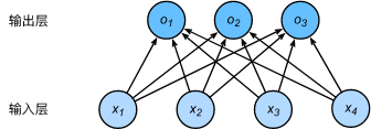
输入的图像高宽均为2像素,色彩为灰度。图像的4像素分别记为x1,x2,x3,x4。
假设真实值标签为猫、狗或鸡,这些标签对应离散值为y1,y2,y3。
权重矢量
o1 = x1w11 + x2w21 + x3w31 + x4w41 + b1
o2 = x2w12 + x2w22 + x3w22 + x4w42 + b2
o3 = x3w13 + x2w23 + x3w33 + x4w43 + b3
神经网络图
每个输出o1,o2,o3计算都要依赖于所有的输入x1,x2,x3,x4,softmax回归输出层也是一个全连接层
将输出值oi当预测类别是i的置信度,并将最大的输出所对应的类作为预测输出(argimaxoi)。
输出:
softmax通过【ˆy1,ˆy2,ˆy3 = softmax(o1,o2,o3)】将输出值变为值为正且和为1的概率分布。其中,ˆy1 =
ˆy3 =
模型训练和预测
在训练好softmax回归模型后,给定任一样本特征,就可以预测每个输出类别的概率。通常,我们把预测概率最大的类别作为输出类别。如果它与真实类别(标签)一致,说明这次预测是正确的。在3.6节的实验中,我们将使用准确率(accuracy)来评价模型的表现。它等于正确预测数量与总预测数量之比。
获取Fashion-MNIST训练集和读取数据
softmax从零开始实现
1 import torch
2 import torchvision
3 import numpy as np
4 import sys
5 sys.path.append("/home/kesci/input")
6 import d2lzh1981 as d2l
7
8 print(torch.__version__)
9 print(torchvision.__version__)
获取训练集数据和测试集数据
1 batch_size = 256
2 train_iter, test_iter = d2l.load_data_fashion_mnist(batch_size, root='/home/kesci/input/FashionMNIST2065')
模型参数初始化
1 num_inputs = 784
2 print(28*28)
3 num_outputs = 10
4
5 W = torch.tensor(np.random.normal(0, 0.01, (num_inputs, num_outputs)), dtype=torch.float)
6 b = torch.zeros(num_outputs, dtype=torch.float
1 W.requires_grad_(requires_grad=True)
2 b.requires_grad_(requires_grad=True)
对多维Tensor按维度操作
1 X = torch.tensor([[1, 2, 3], [4, 5, 6]])
2 print(X.sum(dim=0, keepdim=True))  # dim为0,按照相同的列求和,并在结果中保留列特征
3 print(X.sum(dim=1, keepdim=True))  # dim为1,按照相同的行求和,并在结果中保留行特征
4 print(X.sum(dim=0, keepdim=False)) # dim为0,按照相同的列求和,不在结果中保留列特征
5 print(X.sum(dim=1, keepdim=False)) # dim为1,按照相同的行求和,不在结果中保留行特征
定义softmax操作 ˆyj = exp(oj) ⁄ ∑ 3i=1 exp(oi)
1 def softmax(X):
2     X_exp = X.exp()
3     partition = X_exp.sum(dim=1, keepdim=True)
4     # print("X size is ", X_exp.size())
5     # print("partition size is ", partition, partition.size())
6     return X_exp / partition  # 这里应用了广播机制
1 X = torch.rand((2, 5))
2 X_prob = softmax(X)
3 print(X_prob, '\n', X_prob.sum(dim=1))
softmax回归模型 o(i) = x(i) W + b , ˆy(i) = softmax(o(i)).
1 def net(X):
2     return softmax(torch.mm(X.view((-1, num_inputs)), W) + b)
定义损失函数
1 y_hat = torch.tensor([[0.1, 0.3, 0.6], [0.3, 0.2, 0.5]])
2 y = torch.LongTensor([0, 2])
3 y_hat.gather(1, y.view(-1, 1))
1 def cross_entropy(y_hat, y):
2     return - torch.log(y_hat.gather(1, y.view(-1, 1)))
定义准确率
1 def accuracy(y_hat, y):
2     return (y_hat.argmax(dim=1) == y).float().mean().item()
1 print(accuracy(y_hat, y))
1 # 本函数已保存在d2lzh_pytorch包中方便以后使用。该函数将被逐步改进:它的完整实现将在“图像增广”一节中描述
2 def evaluate_accuracy(data_iter, net):
3     acc_sum, n = 0.0, 0
4     for X, y in data_iter:
5         acc_sum += (net(X).argmax(dim=1) == y).float().sum().item()
6         n += y.shape[0]
7     return acc_sum / n
1 print(evaluate_accuracy(test_iter , net))
训练模型
 1 num_epochs, lr = 5, 0.1
 2
 3 # 本函数已保存在d2lzh_pytorch包中方便以后使用
 4 def train_ch3(net, train_iter, test_iter, loss, num_epochs, batch_size,
 5               params=None, lr=None, optimizer=None):
 6     for epoch in range(num_epochs):
 7         train_l_sum, train_acc_sum, n = 0.0, 0.0, 0
 8         for X, y in train_iter:
 9             y_hat = net(X)
10             l = loss(y_hat, y).sum()
11
12             # 梯度清零
13             if optimizer is not None:
14                 optimizer.zero_grad()
15             elif params is not None and params[0].grad is not None:
16                 for param in params:
17                     param.grad.data.zero_()
18
19             l.backward()
20             if optimizer is None:
21                 d2l.sgd(params, lr, batch_size)
22             else:
23                 optimizer.step()
24
25
26             train_l_sum += l.item()
27             train_acc_sum += (y_hat.argmax(dim=1) == y).sum().item()
28             n += y.shape[0]
29         test_acc = evaluate_accuracy(test_iter, net)
30         print('epoch %d, loss %.4f, train acc %.3f, test acc %.3f'
31               % (epoch + 1, train_l_sum / n, train_acc_sum / n, test_acc))
32
33 train_ch3(net, train_iter, test_iter, cross_entropy, num_epochs, batch_size, [W, b], lr)
模型预测
模型训练完进行一下预测。演示如何对图像进行分类。给定一系列图像(第三行图像输出),比较一下它们的真实标签(第一行文本输出)和模型预测结果(第二行文本输出)。
1 X, y = iter(test_iter).next()
2
3 true_labels = d2l.get_fashion_mnist_labels(y.numpy())
4 pred_labels = d2l.get_fashion_mnist_labels(net(X).argmax(dim=1).numpy())
5 titles = [true + '\n' + pred for true, pred in zip(true_labels, pred_labels)]
6
7 d2l.show_fashion_mnist(X[0:9], titles[0:9])
- 可以使用softmax回归做多类别分类。与训练线性回归相比,你会发现训练softmax回归的步骤和它非常相似:获取并读取数据、定义模型和损失函数并使用优化算法训练模型。事实上,绝大多数深度学习模型的训练都有着类似的步骤。
三、多层感知机
知识点记录
在深度学习中主要关注多层模型,线性回归和softmax回归是单层神经网络,多层感知机是多层神经网络
隐藏层
多层感知机在单层神经网络的基础上引入了一道多的隐藏层,位于输入层和输出层之间。
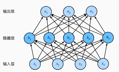 其中含有一个隐藏层,该层中有5个隐藏单元。输入层不涉及计算,所以图所示感知机层数为2.隐藏层中的神经元和输入层中的各个输入完全链接,输出层中的神经元和隐藏层中的各个神经元也完全连接,因此,多层感知机中的隐藏层和输出层都是全连接层。
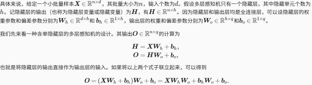
由式子看出,神经网络引入了隐藏层,依然等价于一个单层神经网络:其中输出权重参数为WhWo,偏差参数为bhWo + bo
激活函数
多层感知机
含有至少一个隐藏层的由全连接层组成的神经网络,且每个隐藏层的输出通过记过函数进行变换。多层感知机的层数和各隐藏层中隐藏单元个数都是超参数。以单隐藏层为例:H =Ø(XWh + bh), O = HWo +bo ,
小结
- 多层感知机在输出层与输入层之间加入了一个或多个全连接隐藏层,并通过激活函数对隐藏层输出进行变换。
- 常用的激活函数包括ReLU函数、sigmoid函数和tanh函数。
1 import torch
2 import numpy as np
3 import sys
4 sys.path.append("/home/kesci/input")
5 import d2lzh1981 as d2l
6 print(torch.__version__)
获取训练集
1 batch_size = 256
2 train_iter, test_iter = d2l.load_data_fashion_mnist(batch_size,root='/home/kesci/input/FashionMNIST2065')
 1 num_inputs, num_outputs, num_hiddens = 784, 10, 256
 2
 3 W1 = torch.tensor(np.random.normal(0, 0.01, (num_inputs, num_hiddens)), dtype=torch.float)
 4 b1 = torch.zeros(num_hiddens, dtype=torch.float)
 5 W2 = torch.tensor(np.random.normal(0, 0.01, (num_hiddens, num_outputs)), dtype=torch.float)
 6 b2 = torch.zeros(num_outputs, dtype=torch.float)
 7
 8 params = [W1, b1, W2, b2]
 9 for param in params:
10     param.requires_grad_(requires_grad=True)
定义激活函数
1 def relu(X):
2     return torch.max(input = X, other=torch.tensor(0,0))
定义网络
1 def net(X):
2     X = X.view((-1, num_inputs))
3     H = relu(torch.matmul(X, W1) + b1)
4     return torch.matmul(H, W2) + b2
1 loss = torch.nn.CrossEntropyLoss()
训练
 1 num_epochs, lr = 5, 100.0
 2 # def train_ch3(net, train_iter, test_iter, loss, num_epochs, batch_size,
 3 #               params=None, lr=None, optimizer=None):
 4 #     for epoch in range(num_epochs):
 5 #         train_l_sum, train_acc_sum, n = 0.0, 0.0, 0
 6 #         for X, y in train_iter:
 7 #             y_hat = net(X)
 8 #             l = loss(y_hat, y).sum()
 9 #
10 #             # 梯度清零
11 #             if optimizer is not None:
12 #                 optimizer.zero_grad()
13 #             elif params is not None and params[0].grad is not None:
14 #                 for param in params:
15 #                     param.grad.data.zero_()
16 #
17 #             l.backward()
18 #             if optimizer is None:
19 #                 d2l.sgd(params, lr, batch_size)
20 #             else:
21 #                 optimizer.step()  # “softmax回归的简洁实现”一节将用到
22 #
23 #
24 #             train_l_sum += l.item()
25 #             train_acc_sum += (y_hat.argmax(dim=1) == y).sum().item()
26 #             n += y.shape[0]
27 #         test_acc = evaluate_accuracy(test_iter, net)
28 #         print('epoch %d, loss %.4f, train acc %.3f, test acc %.3f'
29 #               % (epoch + 1, train_l_sum / n, train_acc_sum / n, test_acc))
30
31 d2l.train_ch3(net, train_iter, test_iter, loss, num_epochs, batch_size, params, lr)

