第二次作业：卷积神经网络 part 2

第一部分问题总结

MobileNetV2的参数为什么比MobileNetV1要少很多？
shortcut连接是干嘛的？

第二部分论文阅读心得

《MobileNets: Efficient Convolutional Neural Networks for Mobile Vision Applications》《用于移动视觉应用程序的高效卷积神经网络》

传统卷积神经网络内存需求大、运算量大、导致无法在移动设备上以及嵌入式设备上运行。谷歌针对手机等嵌入式设备提出了一类有效的模型MobileNets。主要的思想就是卷积核的巧妙分解，实现有效的减少网络参数。

Abstract

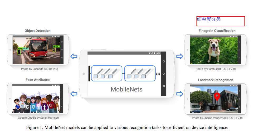
谷歌提出了我们提出了一类有效的模型称为移动和嵌入式视觉应用程序的MobileNets。MobileNets基于一种流线型的架构，使用深度可分离的卷积来构建轻量级的深度神经网络。引入了两个简单的全局超参数，可以有效地在延迟和准确性之间进行权衡。这些超参数允许模型构建者根据问题的约束条件为他们的应用程序选择合适大小的模型。演示了mobilenet的有效性跨广泛的应用和用例，包括对象检测，细粒度分类，人脸属性和大规模地理定位。

Introduction

这部分是说，随着深度学习的发展，卷积神经网络变得越来越普遍。当前发展的总体趋势是，通过更深和更复杂的网络来得到更高的精度，但是这种网络往往在模型大小和运行速度上没多大优势。一些嵌入式平台上的应用比如机器人和自动驾驶，它们的硬件资源有限，就十分需要一种轻量级、低延迟（同时精度尚可接受）的网络模型，这就是本文的主要工作。

α是控制卷积层卷积核个数，β是控制输入图像的大小，人为设定的。

MobileNet Architecture
- Depthwise Separable Convolution （深度可分离卷积）

如下图所示为传统的卷积，输入图像深度（channel）为3的特征矩阵，利用四个卷积核进行卷积，每个卷积核的深度(channel)和输入的特征矩阵深度是相同的。即卷积核的深度为3。每个卷积核的channel和输入图像矩阵的三个channel相对应进行运算。输出特征矩阵的深度与卷积核的个数有关，卷积核的个数为4，即输出特征矩阵的深度也是4。

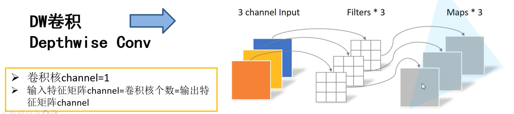
在DW(Depthwise Convolution)卷积中，如下图所示，相同条件下，卷积核的个数是3，输出特征矩阵的深度也是3。卷积核的深度是1，即每个卷积核只跟输入图像矩阵的一个channel进行运算得到一个输出矩阵channel。

Depthwise Separable Convolution(深度可分离卷积)由两部分组成一个是上面的DW卷积，一个是PW卷积，即(Pointwise Convolution)。PW卷积与传统的卷积相比就是卷积核的大小为1x1。

那么使用深度可分离卷积与传统的卷积相比到底能节省多少参数呢。

D_F表示输入特征矩阵的高和宽

D_K表示卷积核的大小

M代表输入特征矩阵的深度

N代表卷积核的个数，也代表输出特征矩阵的深度（在DW卷积中，M=N）

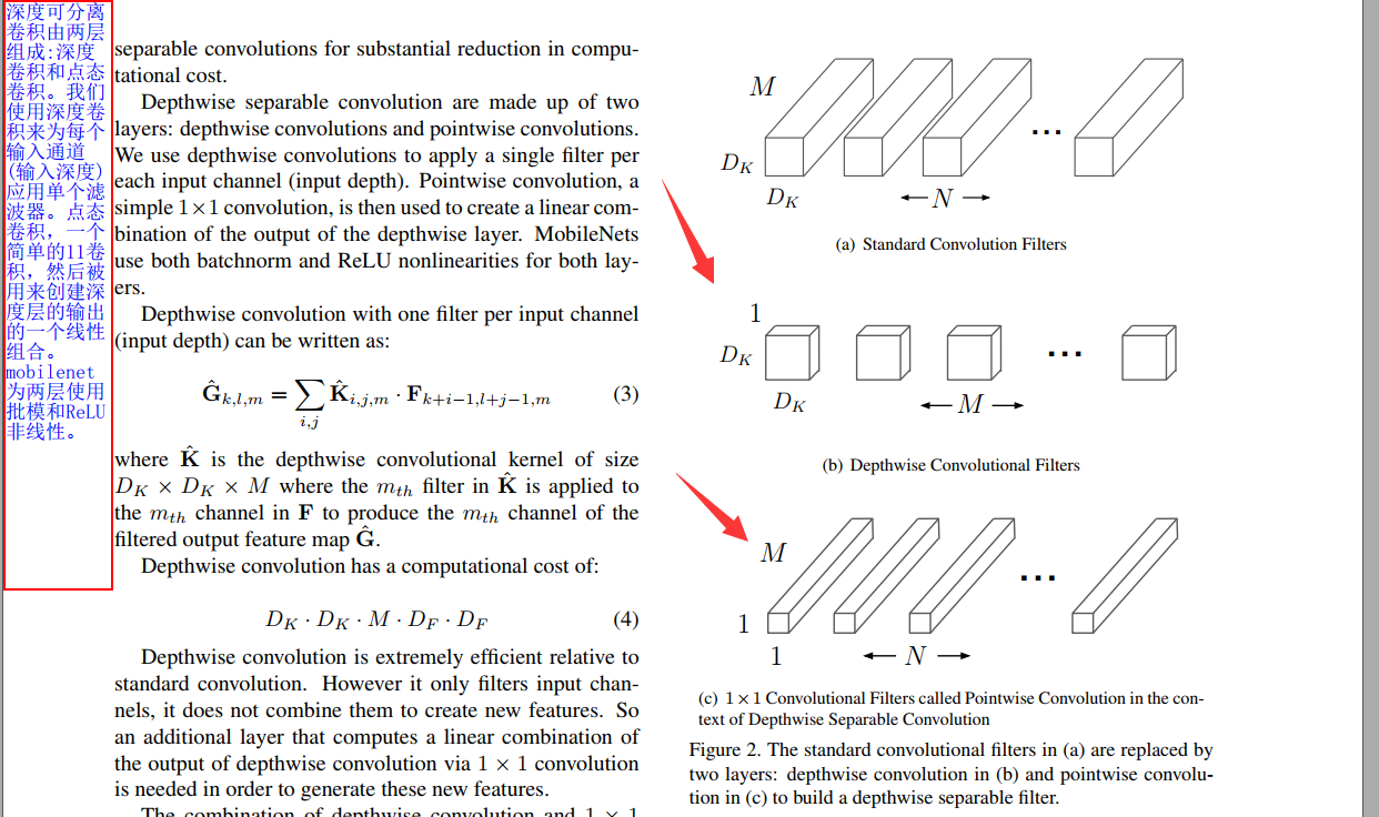
上图是论文中的描述，跟下图的描述是一回事，下图的图片展示得更加清晰。

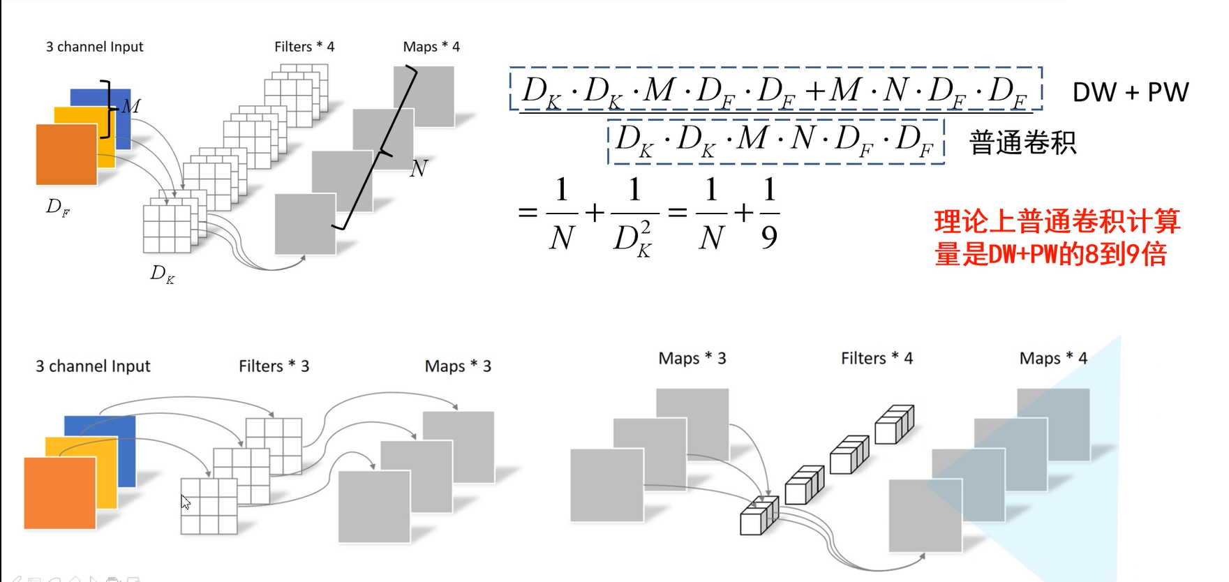
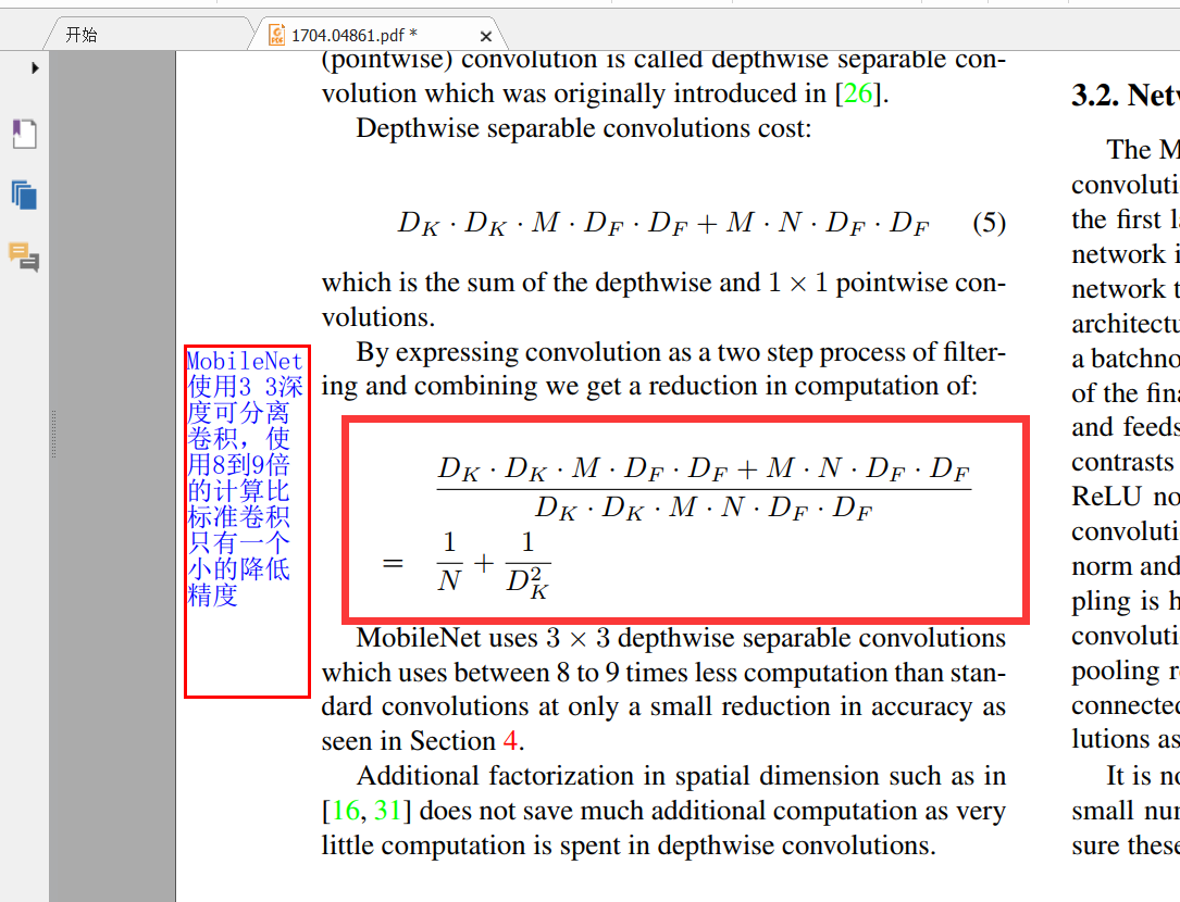
如上图所示，普通卷积的计算量就是\(D_F*D_F*M*N*D_K*D_K\)默认stride为1，输入特征矩阵的计算量就是\(D_F*D_F\)。对于深度可分离卷积，其计算量包含Depthwise Conv和Pointwise Conv。DW卷积的计算量就是\(D_K*D_K*M*D_F*D_F(N=1)\)，PW卷积的计算量就是\(D_F*D_F*M*N\) (\(D_K=1因为卷积核的大小为1\))。由于MobileNets使用了大量的3 × 3的卷积核，两种卷积的计算量对比可以看出普通卷积的计算量是DW+PW的8-9倍左右。

下图是论文中的公式：

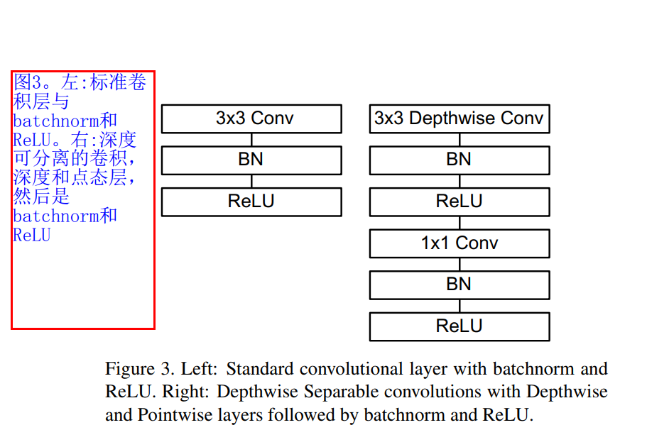
下图是论文中的MobileNetV1 Body Architecture 。MobileNets结构建立在上述深度可分解卷积中（只有第一层是标准卷积）。该网络允许我们探索网络拓扑，找到一个适合的良好网络。其具体架构在Table 1说明。除了最后的全连接层，所有层后面跟了batchnorm和ReLU，最终输入到softmax进行分类。图3对比了标准卷积和分解卷积的结构，二者都附带了BN和ReLU层。按照作者的计算方法，MobileNets总共28层（1 + 2 × 13 + 1 = 28）。

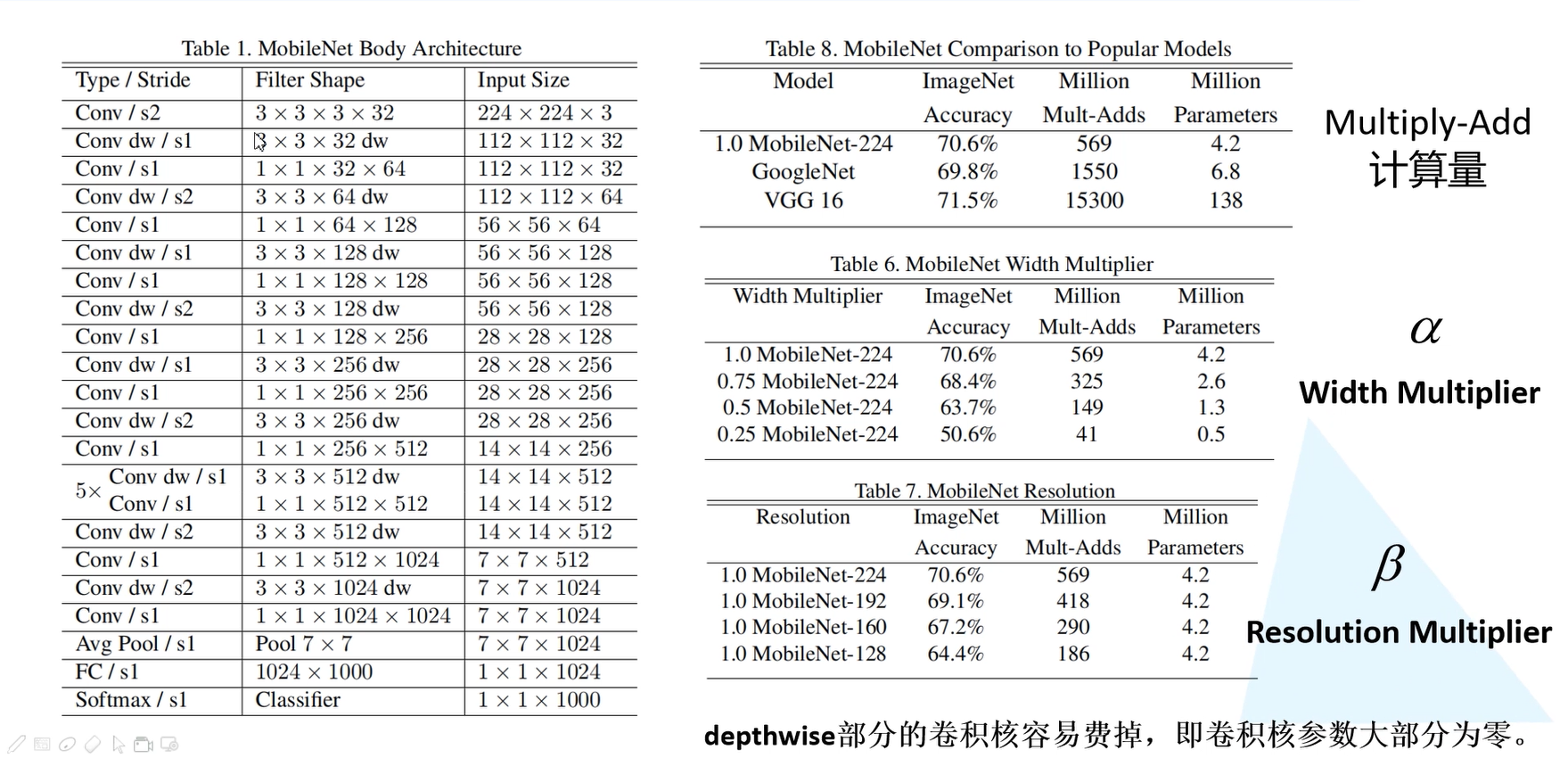
例如第一行的Conv/s2代表普通卷积，步长为2，3x3x3x32表示卷积核的大小为3x3，深度为3，也就是输入特征矩阵有3个通道，一共有32个卷积核。第二行Conv/dw/s1代表dw卷积，步长为1，卷积核的大小3x3,深度为 1，32表示卷积核的个数也就是输出特征矩阵的深度。下面的与上述的类似，就是将一些卷积进行简单的串行连接。与VGG网络相似。

从上图可以看出MobileNetV1网络在ImageNets数据集上的准确率是70.6%。相对于GooleNet增加了0.8%，相对于VGG降低了0.9%。但是其模型参数大概只有VGG网络的1/32。

α表示卷积核个数的一个倍率，也就是控制卷积核的个数，对应Table 6中的Width Multiplier。可以看出当卷积核的个数不断减少的时候，其准确率也不断下降。但是模型参数也减少了很多。

β表示输入的图像大小，即对应Table 7中的Resolution。当输入图像越小时，其准确率越小。计算量也越少。

depthwise部分的卷积核容易废掉，即卷积核的参数大部分为0。MobileNetV2做了进一步改善。（这里不太懂。。。。。）

《MobileNetV2: Inverted Residuals and Linear Bottlenecks 》《倒残差和线性瓶颈》

本文是MobileNets的第二版。第一版中，MobileNets全面应用了Depth-wise Seperable Convolution并提出两个超参来控制网络容量，在保持移动端可接受的模型复杂性的基础上达到了相当的精度。而第二版中，MobileNets应用了新的单元：Inverted residual with linear bottleneck，主要的改动是添加了线性Bottleneck和将skip-connection转移到低维bottleneck层。

MobileNetV2网络相比MobileNetV1网络，准确率更高，模型更小。网络中的亮点：Inverted Residuals(倒残差结构)和Linear Bottlenecks。

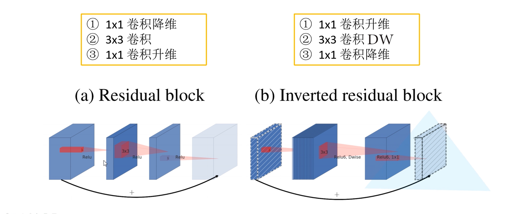
在ResNet网络残差结构中，对于输入特征矩阵我们采用1x1的卷积核进行压缩，减少输入特征矩阵的channel。然后利用3x3的卷积核进行卷积处理，最后利用1x1的卷积核进行扩充channel。就形成了一个两头大中间小的结构。而倒残差结构与此相反。

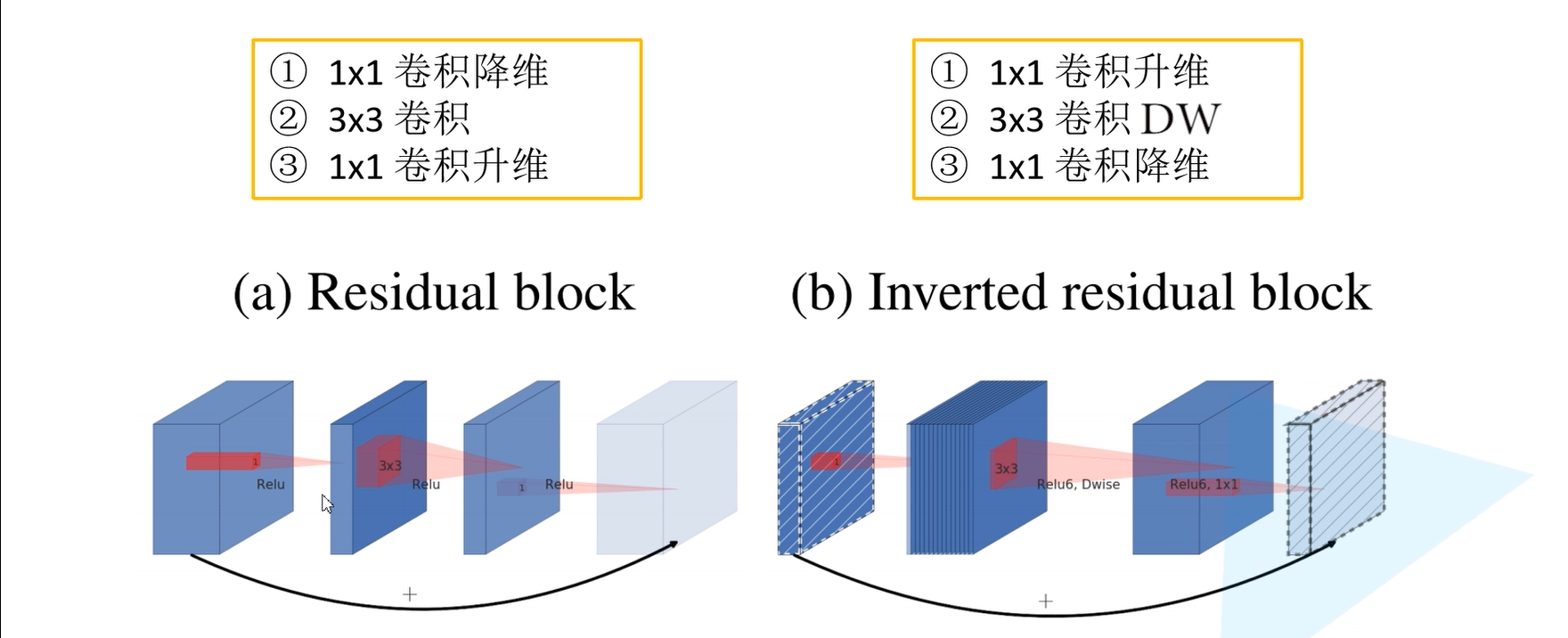
在普通的残差网络结构中，采用的激活函数是ReLU激活函数，而在倒残差网络结构中使用的是ReLU6激活函数。

普通的ReLU函数当输入值小于0时，默认置0，当输入值大于0的时候，不对它进行处理，ReLU6中对输入值大于6时，就维持在6。

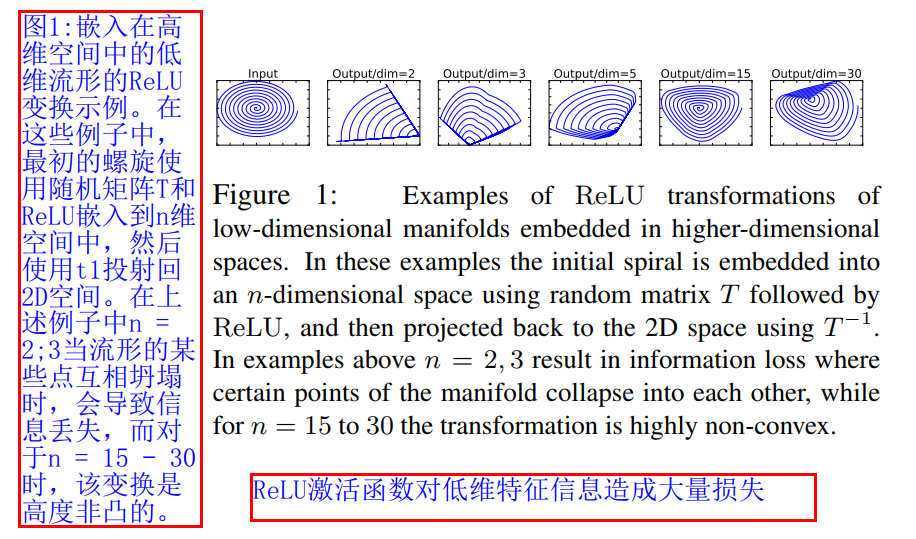
Linear Bottlenecks ：在原论文中针对倒残差结构的最后一个1x1卷积层。它使用了线性激活函数，而不是ReLU激活函数。线性激活函数可以避免出现特征信息的大量流失。

上图中，利用MxN的矩阵B将张量（2D，即N=2）变换到M维的空间中，通过ReLUctant后（y=ReLU(Bx)），再用此矩阵之逆恢复原来的张量。可以看到，当M较小时，恢复后的张量坍缩严重，M较大时则恢复较好。

这意味着，在较低维度的张量表示（兴趣流形）上进行ReLU等线性变换会有很大的信息损耗。因而本文提出使用线性变换替代Bottleneck的激活层，而在需要激活的卷积层中，使用较大的M使张量在进行激活前先扩张，整个单元的输入输出是低维张量，而中间的层则用较高维的张量。

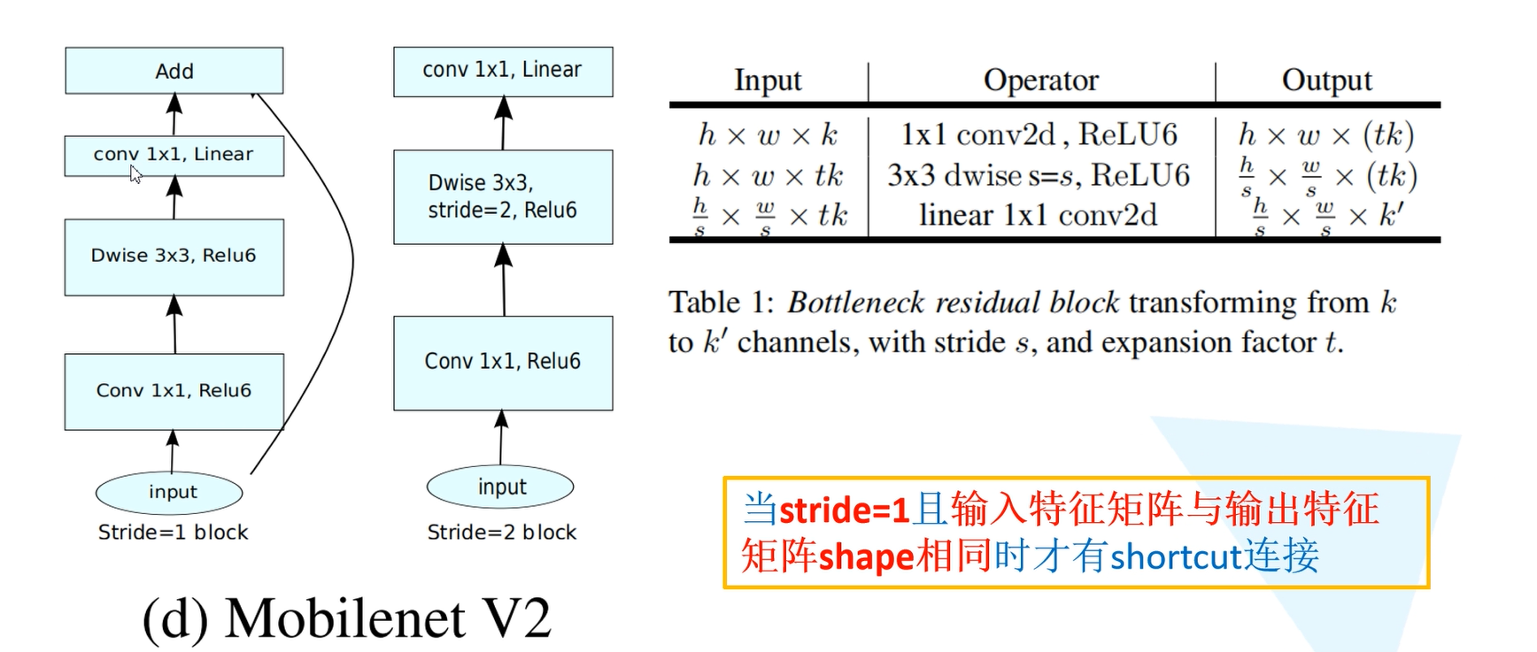
h x w x k表示输入特征矩阵的高、宽和深度。1x1 conv2d表示用1x1的卷积核进行升维的处理。

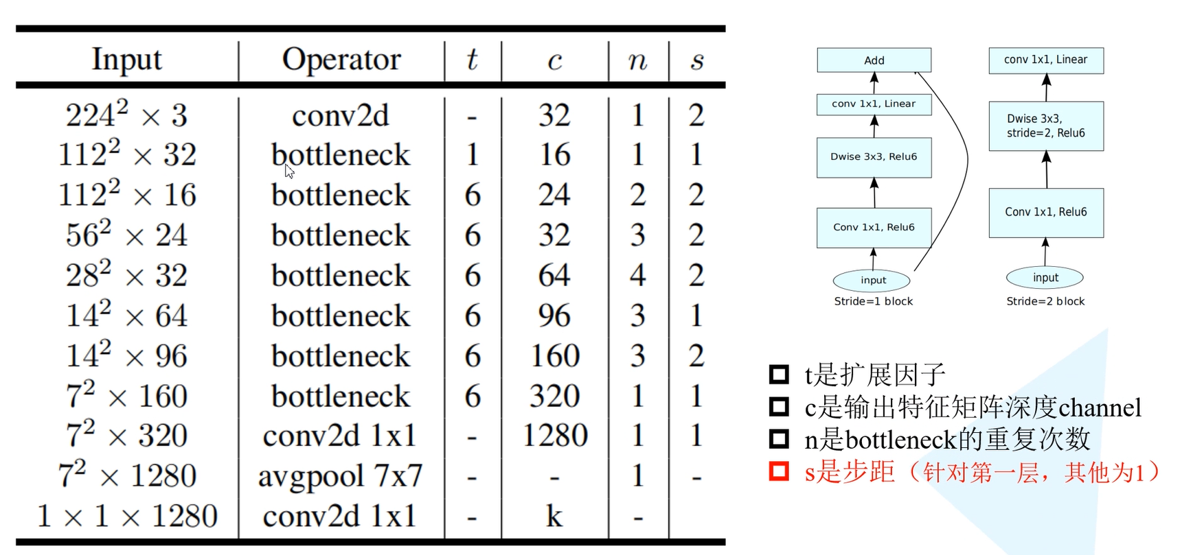
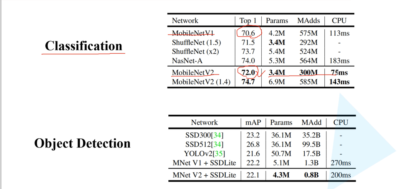
t代表单元的扩张系数，c代表channel数，n为单元重复个数，s为stride数。可见，网络整体上遵循了重复相同单元和加深则变宽等设计范式。下图是MobileNetV2在分类和目标检测领域相对于MobileNetV1网络和其他网络结构的性能对比。

《HybridSN: Exploring 3D-2D CNN Feature Hierarchy for Hyperspectral Image Classification 》《HybridSN:探索CNN 3D-2D功能用于高光谱图像分类的层次结构》

本篇论文主要是构建了一个混合网络解决高光谱图像分类问题，首先用3D卷积，然后使用2D卷积来实现。

主要原因：仅使用2D-CNN或3D-CNN分别存在缺失通道关系信息或模型非常复杂等缺点。这也阻碍了这些方法在高光谱图像上取得更好的精度。主要原因是高光谱图像是体积数据，也有光谱维数。仅凭2D-CNN无法从光谱维度中提取出具有良好鉴别能力的feature maps。

定义HybridSN类

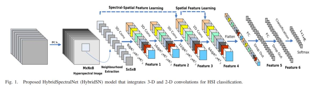
如上图所示，将3D-CNN和2D-CNN层组合到假想模型中，使其充分利用光谱和空间特征地图，以达到最大可能的精度。

三维卷积部分：

conv1：（1, 30, 25, 25）， 8个 7x3x3 的卷积核 ==>（8, 24, 23, 23）

conv2：（8, 24, 23, 23）， 16个 5x3x3 的卷积核 ==>（16, 20, 21, 21）

conv3：（16, 20, 21, 21），32个 3x3x3 的卷积核 ==>（32, 18, 19, 19）

接下来要进行二维卷积，因此把前面的 32*18 reshape 一下，得到（576, 19, 19）

二维卷积：（576, 19, 19） 64个 3x3 的卷积核，得到（64, 17, 17）

接下来是一个 flatten 操作，变为 18496 维的向量，

接下来依次为256，128节点的全连接层，都使用比例为0.4的 Dropout，

最后输出为 16 个节点，是最终的分类类别数

在2D- cnn中，输入数据与2D核进行卷积。卷积是通过计算输入数据和核函数的点积的和来实现的。内核跨越输入数据以覆盖整个空间维度。通过激活函数将卷积特征引入到模型中。在二维卷积。第i层第j个feature map空间位置(x, y)的激活值记为vi,j，方程如下

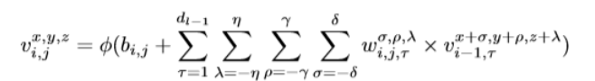
在HSI数据模型中，利用三维核在输入层的多个连续频带上生成卷积层的特征图;这捕获了光谱信息。在三维卷积中，第i层第j个feature map空间位置(x, y, z)的激活值记为，yz，方程如下

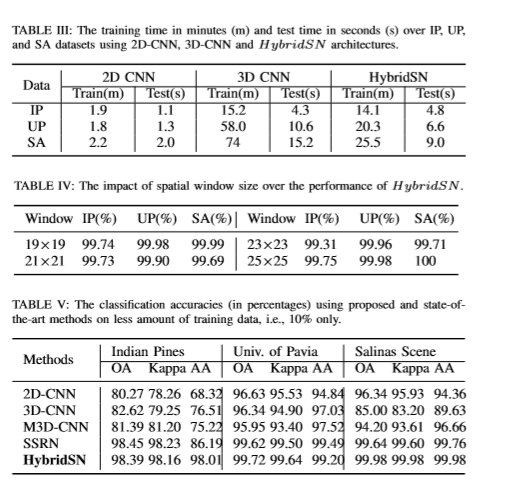
由于光谱波段中增加的冗余，2D-CNN比3D-CNN在Salinas场景数据集上表现更好。此外，SSRN和HybridSN的性能一直远优于M3D-CNN。很明显，与混合的3D和2D卷积相比，3D或2D卷积的alonc不能代表高度分辨力的特征。

使用SVM、2D-CNN、3D-CNN对一个示例高光谱图像的分类图如图所示。M3D-CNN, SSRN和HubridSN方法。SSRN和hybrid的分类图质量明显优于其他方法。在SSRN和hybrid中，hybrid在小段内生成的地图要优于SSRN。

本论文主要提出的hybrid dsn模型基本上是将空间光谱和光谱的互补信息分别以三维卷积和二维卷积的形式结合在一起。数据集与目前最先进的方法进行了比较，验证了该方法的优越性。该模型比3D-CNN模型的计算效率更高。在小的训练数据上也显示出了优越的性能。

第三部分代码练习

《MobileNets: Efficient Convolutional Neural Networks for Mobile Vision Applications》

import torch
import torch.nn as nn
import torch.nn.functional as F
import torchvision
import torchvision.transforms as transforms
import matplotlib.pyplot as plt
import numpy as np
import torch.optim as optim

class Block(nn.Module):
    '''Depthwise conv + Pointwise conv'''
    def __init__(self, in_planes, out_planes, stride=1):
        super(Block, self).__init__()
        # Depthwise 卷积，3*3 的卷积核，分为 in_planes，即各层单独进行卷积
        self.conv1 = nn.Conv2d(in_planes, in_planes, kernel_size=3, stride=stride, padding=1, groups=in_planes, bias=False)
        self.bn1 = nn.BatchNorm2d(in_planes)
        # Pointwise 卷积，1*1 的卷积核
        self.conv2 = nn.Conv2d(in_planes, out_planes, kernel_size=1, stride=1, padding=0, bias=False)
        self.bn2 = nn.BatchNorm2d(out_planes)

    def forward(self, x):
        out = F.relu(self.bn1(self.conv1(x)))
        out = F.relu(self.bn2(self.conv2(out)))
        return out

创建 DataLoader

# 使用GPU训练，可以在菜单 "代码执行工具" -> "更改运行时类型" 里进行设置
device = torch.device("cuda:0" if torch.cuda.is_available() else "cpu")

transform_train = transforms.Compose([
    transforms.RandomCrop(32, padding=4),
    transforms.RandomHorizontalFlip(),
    transforms.ToTensor(),
    transforms.Normalize((0.4914, 0.4822, 0.4465), (0.2023, 0.1994, 0.2010))])

transform_test = transforms.Compose([
    transforms.ToTensor(),
    transforms.Normalize((0.4914, 0.4822, 0.4465), (0.2023, 0.1994, 0.2010))])

trainset = torchvision.datasets.CIFAR10(root='./data', train=True,  download=True, transform=transform_train)
testset  = torchvision.datasets.CIFAR10(root='./data', train=False, download=True, transform=transform_test)

trainloader = torch.utils.data.DataLoader(trainset, batch_size=128, shuffle=True, num_workers=2)
testloader = torch.utils.data.DataLoader(testset, batch_size=128, shuffle=False, num_workers=2)

创建 MobileNetV1 网络

32×32×3 ==>

32×32×32 ==> 32×32×64 ==> 16×16×128 ==> 16×16×128 ==>

8×8×256 ==> 8×8×256 ==> 4×4×512 ==> 4×4×512 ==>

2×2×1024 ==> 2×2×1024

接下来为均值 pooling ==> 1×1×1024

最后全连接到 10个输出节点

class MobileNetV1(nn.Module):
    # (128,2) means conv planes=128, stride=2
    cfg = [(64,1), (128,2), (128,1), (256,2), (256,1), (512,2), (512,1), 
           (1024,2), (1024,1)]

    def __init__(self, num_classes=10):
        super(MobileNetV1, self).__init__()
        self.conv1 = nn.Conv2d(3, 32, kernel_size=3, stride=1, padding=1, bias=False)
        self.bn1 = nn.BatchNorm2d(32)
        self.layers = self._make_layers(in_planes=32)
        self.linear = nn.Linear(1024, num_classes)

    def _make_layers(self, in_planes):
        layers = []
        for x in self.cfg:
            out_planes = x[0]
            stride = x[1]
            layers.append(Block(in_planes, out_planes, stride))
            in_planes = out_planes
        return nn.Sequential(*layers)

    def forward(self, x):
        out = F.relu(self.bn1(self.conv1(x)))
        out = self.layers(out)
        out = F.avg_pool2d(out, 2)
        out = out.view(out.size(0), -1)
        out = self.linear(out)
        return out

实例化网络

# 网络放到GPU上
net = MobileNetV1().to(device)
criterion = nn.CrossEntropyLoss()
optimizer = optim.Adam(net.parameters(), lr=0.001)

模型训练

for epoch in range(10):  # 重复多轮训练
    for i, (inputs, labels) in enumerate(trainloader):
        inputs = inputs.to(device)
        labels = labels.to(device)
        # 优化器梯度归零
        optimizer.zero_grad()
        # 正向传播 +　反向传播 + 优化 
        outputs = net(inputs)
        loss = criterion(outputs, labels)
        loss.backward()
        optimizer.step()
        # 输出统计信息
        if i % 100 == 0:   
            print('Epoch: %d Minibatch: %5d loss: %.3f' %(epoch + 1, i + 1, loss.item()))

print('Finished Training')

模型测试

correct = 0
total = 0
for data in testloader:
    images, labels = data
    images, labels = images.to(device), labels.to(device)
    outputs = net(images)
    _, predicted = torch.max(outputs.data, 1)
    total += labels.size(0)
    correct += (predicted == labels).sum().item()

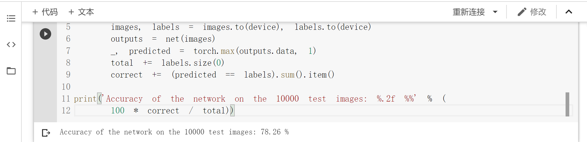
print('Accuracy of the network on the 10000 test images: %.2f %%' % (
    100 * correct / total))

《MobileNetV2: Inverted Residuals and Linear Bottlenecks》

MobileNet V1 的主要问题：结构非常简单，但是没有使用RestNet里的residual learning；另一方面，Depthwise Conv确实是大大降低了计算量，但实际中，发现不少训练出来的kernel是空的。下面就是 Inverted residual block 部分的代码，主要思路就是:

expand + Depthwise + Pointwise 其中，expand就是增大feature map数量的意思。需要指出的是，当步长为1的时候，要加一个 shortcut；步长为2的时候，目的是降低feature map尺寸，就不需要加 shortcut 了。

import torch
import torch.nn as nn
import torch.nn.functional as F
import torchvision
import torchvision.transforms as transforms
import matplotlib.pyplot as plt
import numpy as np
import torch.optim as optim

class Block(nn.Module):
    '''expand + depthwise + pointwise'''
    def __init__(self, in_planes, out_planes, expansion, stride):
        super(Block, self).__init__()
        self.stride = stride
        # 通过 expansion 增大 feature map 的数量
        planes = expansion * in_planes
        self.conv1 = nn.Conv2d(in_planes, planes, kernel_size=1, stride=1, padding=0, bias=False)
        self.bn1 = nn.BatchNorm2d(planes)
        self.conv2 = nn.Conv2d(planes, planes, kernel_size=3, stride=stride, padding=1, groups=planes, bias=False)
        self.bn2 = nn.BatchNorm2d(planes)
        self.conv3 = nn.Conv2d(planes, out_planes, kernel_size=1, stride=1, padding=0, bias=False)
        self.bn3 = nn.BatchNorm2d(out_planes)

        # 步长为 1 时，如果 in 和 out 的 feature map 通道不同，用一个卷积改变通道数
        if stride == 1 and in_planes != out_planes:
            self.shortcut = nn.Sequential(
                nn.Conv2d(in_planes, out_planes, kernel_size=1, stride=1, padding=0, bias=False),
                nn.BatchNorm2d(out_planes))
        # 步长为 1 时，如果 in 和 out 的 feature map 通道相同，直接返回输入
        if stride == 1 and in_planes == out_planes:
            self.shortcut = nn.Sequential()

    def forward(self, x):
        out = F.relu(self.bn1(self.conv1(x)))
        out = F.relu(self.bn2(self.conv2(out)))
        out = self.bn3(self.conv3(out))
        # 步长为1，加 shortcut 操作
        if self.stride == 1:
            return out + self.shortcut(x)
        # 步长为2，直接输出
        else:
            return out

创建 MobileNetV2 网络

注意，因为 CIFAR10 是 32*32，因此，网络有一定修改。

class MobileNetV2(nn.Module):
    # (expansion, out_planes, num_blocks, stride)
    cfg = [(1,  16, 1, 1),
           (6,  24, 2, 1), 
           (6,  32, 3, 2),
           (6,  64, 4, 2),
           (6,  96, 3, 1),
           (6, 160, 3, 2),
           (6, 320, 1, 1)]

    def __init__(self, num_classes=10):
        super(MobileNetV2, self).__init__()
        self.conv1 = nn.Conv2d(3, 32, kernel_size=3, stride=1, padding=1, bias=False)
        self.bn1 = nn.BatchNorm2d(32)
        self.layers = self._make_layers(in_planes=32)
        self.conv2 = nn.Conv2d(320, 1280, kernel_size=1, stride=1, padding=0, bias=False)
        self.bn2 = nn.BatchNorm2d(1280)
        self.linear = nn.Linear(1280, num_classes)

    def _make_layers(self, in_planes):
        layers = []
        for expansion, out_planes, num_blocks, stride in self.cfg:
            strides = [stride] + [1]*(num_blocks-1)
            for stride in strides:
                layers.append(Block(in_planes, out_planes, expansion, stride))
                in_planes = out_planes
        return nn.Sequential(*layers)

    def forward(self, x):
        out = F.relu(self.bn1(self.conv1(x)))
        out = self.layers(out)
        out = F.relu(self.bn2(self.conv2(out)))
        out = F.avg_pool2d(out, 4)
        out = out.view(out.size(0), -1)
        out = self.linear(out)
        return out

创建 DataLoader

#使用GPU训练，可以在菜单 "代码执行工具" -> "更改运行时类型" 里进行设置
device = torch.device("cuda:0" if torch.cuda.is_available() else "cpu")

transform_train = transforms.Compose([
    transforms.RandomCrop(32, padding=4),
    transforms.RandomHorizontalFlip(),
    transforms.ToTensor(),
    transforms.Normalize((0.4914, 0.4822, 0.4465), (0.2023, 0.1994, 0.2010))])

transform_test = transforms.Compose([
    transforms.ToTensor(),
    transforms.Normalize((0.4914, 0.4822, 0.4465), (0.2023, 0.1994, 0.2010))])

trainset = torchvision.datasets.CIFAR10(root='./data', train=True,  download=True, transform=transform_train)
testset  = torchvision.datasets.CIFAR10(root='./data', train=False, download=True, transform=transform_test)

trainloader = torch.utils.data.DataLoader(trainset, batch_size=128, shuffle=True, num_workers=2)
testloader = torch.utils.data.DataLoader(testset, batch_size=128, shuffle=False, num_workers=2)

实例化网络

# 网络放到GPU上
net = MobileNetV2().to(device)
criterion = nn.CrossEntropyLoss()
optimizer = optim.Adam(net.parameters(), lr=0.001)

模型训练

for epoch in range(10):  # 重复多轮训练
    for i, (inputs, labels) in enumerate(trainloader):
        inputs = inputs.to(device)
        labels = labels.to(device)
        # 优化器梯度归零
        optimizer.zero_grad()
        # 正向传播 +　反向传播 + 优化 
        outputs = net(inputs)
        loss = criterion(outputs, labels)
        loss.backward()
        optimizer.step()
        # 输出统计信息
        if i % 100 == 0:   
            print('Epoch: %d Minibatch: %5d loss: %.3f' %(epoch + 1, i + 1, loss.item()))

print('Finished Training')

模型测试

correct = 0
total = 0

for data in testloader:
    images, labels = data
    images, labels = images.to(device), labels.to(device)
    outputs = net(images)
    _, predicted = torch.max(outputs.data, 1)
    total += labels.size(0)
    correct += (predicted == labels).sum().item()

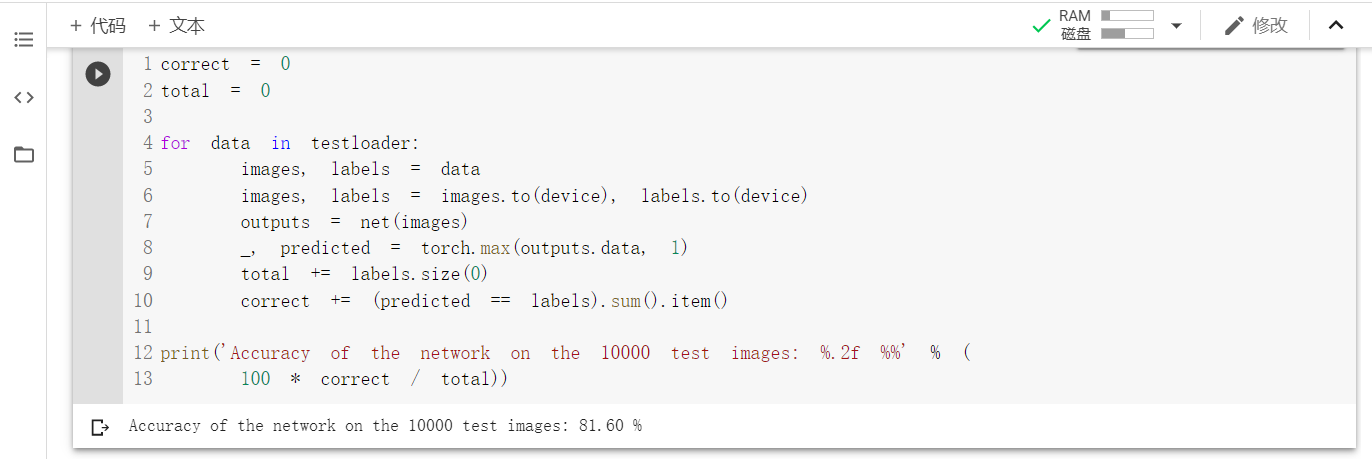
print('Accuracy of the network on the 10000 test images: %.2f %%' % (
    100 * correct / total))

《HybridSN: Exploring 3-D–2-DCNN Feature Hierarchy for Hyperspectral Image Classification》

没弄懂。。。。

class_num = 16
class HybridSN(nn.Module):
  def __init__(self):
    super(HybridSN, self).__init__()
    self.L = 30
    self.S = 25

    self.conv1 = nn.Conv3d(1, 8, kernel_size=(7, 3, 3), stride=1, padding=0)
    self.conv2 = nn.Conv3d(8, 16, kernel_size=(5, 3, 3), stride=1, padding=0)
    self.conv3 = nn.Conv3d(16, 32, kernel_size=(3, 3, 3), stride=1, padding=0)

    inputX = self.get2Dinput()
    inputConv4 = inputX.shape[1] * inputX.shape[2]
    self.conv4 = nn.Conv2d(inputConv4, 64, kernel_size=(3, 3), stride=1, padding=0)

    num = inputX.shape[3]-2 #二维卷积后（64, 17, 17）-->num = 17
    inputFc1 = 64 * num * num
    self.fc1 = nn.Linear(inputFc1, 256) # 64 * 17 * 17 = 18496
    self.fc2 = nn.Linear(256, 128)
    self.fc3 = nn.Linear(128, class_num)
    self.dropout = nn.Dropout(0.4)

  def get2Dinput(self):
    with torch.no_grad():
      x = torch.zeros((1, 1, self.L, self.S, self.S))
      x = self.conv1(x)
      x = self.conv2(x)
      x = self.conv3(x)
    return x

  def forward(self, x):
    x = F.relu(self.conv1(x))
    x = F.relu(self.conv2(x))
    x = F.relu(self.conv3(x))
    x = x.view(x.shape[0], -1, x.shape[3], x.shape[4])
    x = F.relu(self.conv4(x))
    x = x.view(-1, x.shape[1] * x.shape[2] * x.shape[3])
    x = F.relu(self.fc1(x))
    x = self.dropout(x)
    x = F.relu(self.fc2(x))
    x = self.dropout(x)
    x = self.fc3(x)
    return x

posted @ 2020-08-08 08:16 Dingding_lucky 阅读(652) 评论(0) 编辑收藏举报

刷新页面返回顶部

ding_IT

第二次作业：卷积神经网络 part 2

第一部分问题总结

第二部分论文阅读心得

第三部分代码练习

创建 DataLoader

创建 MobileNetV1 网络

实例化网络

模型训练

模型测试

创建 MobileNetV2 网络

创建 DataLoader

实例化网络

模型训练

模型测试

公告

ding_IT

第二次作业：卷积神经网络 part 2

第一部分 问题总结

第二部分 论文阅读心得

第三部分 代码练习

创建 DataLoader

创建 MobileNetV1 网络

实例化网络

模型训练

模型测试

创建 MobileNetV2 网络

创建 DataLoader

实例化网络

模型训练

模型测试

公告

第一部分问题总结

第二部分论文阅读心得

第三部分代码练习