论文笔记(9)-"Personalized Federated Learning with Gaussian Processes"

Personalized Federated Learning with Gaussian Processes

这篇blog不会涉及任何实现细节（因为我没看懂），也不会讲任何该方法的advantages（因为我也没看懂他到底怎么novel），只会说一说这篇文章干了什么事，总之会是一个很朦胧的blog（就装自己懂了吧）。

Motivation

这篇文章它自己提的motivation是“learn effectively across clients even though each client has unique data that is often limited in size”，大致意思就是如何在少量样本下建立一个PFL。然后作者就想到高斯过程（GP）在少样本条件下表现的很好，就想把GP搬到FL里。

Challenges & solutions

non-Gaussian in classification problem

因为FL很多都是分类问题，而在该类问题上得到的marginal distribution不是高斯分布。作者就提出引入服从Pólya-Gamma augmentation分布的变量\(\omega\)来解决。

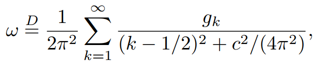
其中\(g_k\sim Gamma(b,1)\)。\(\omega\)满足这样的性质

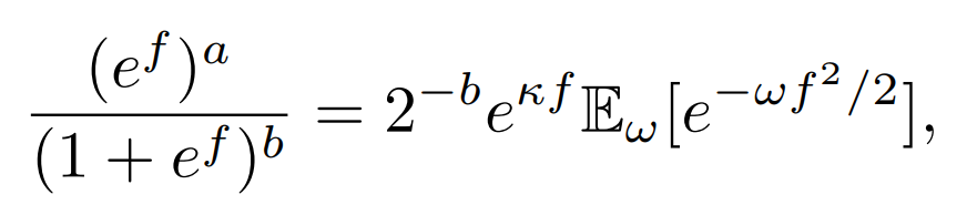
似然可以写成这样形式：

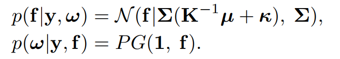
后验是这样的：

Multiclass classification

上面这种Pólya-Gamma augmentation仅适用于二分类的情况，对于Cifar10，Cifar100这种多分类的问题，是不适用的。但是多分类问题可以划分为多个二分类问题，因此作者提出构建一个GP-tree，例如对于Cifar10数据这个GP-tree中应该有10个叶子节点，每一个叶子节点对应一个图片类别。树种的所有非叶子节点都对应一个Pólya-Gamma augmentation的GP。

在文中，作者是通过Kmeans或者Hierarchy cluster来构建树的，具体可以看下代码：

class Split(object):
    # split the node into two or more branches
    # the base class
    def __init__(self, labels, branches=3):
        self.old_to_new = {}
        self.labels = labels
        self.classes = np.unique(labels)
        self.num_classes = self.classes.shape[0]
        self.branches = branches

    def split(self, *args, **kwargs):
        if self.num_classes == 3:
            self.old_to_new[self.classes[0]] = 0
            self.old_to_new[self.classes[1]] = 1
            self.old_to_new[self.classes[2]] = 2
        elif self.num_classes == 2:
            self.old_to_new[self.classes[0]] = 0
            self.old_to_new[self.classes[1]] = 1
        else:
            self.old_to_new[self.classes[0]] = 0
        return self.old_to_new

class ProtoTypeSplit(Split):
    """
    split labels associated with a node to x branches by the prototype of each class.
    close classes should be grouped together
    :param labels: numpy array of the labels
    :param branches: the number of branches
    :param prototype: dictionary of {label: np.array()}
    :param affinity: Metric - “euclidean”, “l1”, “l2”, “manhattan”, “cosine”
    :param linkage: Distance to use between sets of observation: “ward”, “complete”, “average”, “single”
    :return the original classes partitioned to nodes
    """
    def __init__(self, labels, branches, prototype, affinity='cosine', linkage='complete'):
        super().__init__(labels, branches)
        self.affinity = affinity
        self.linkage = linkage
        self.prototype = prototype

    def split(self):

        # hierarchical clustreing
        n_clusters = self.branches
        clustering = AgglomerativeClustering(n_clusters=n_clusters, affinity=self.affinity, linkage=self.linkage)
        lbl_assignment = clustering.fit(list(self.prototype.values())).labels_

        for o, n in zip(self.prototype.keys(), lbl_assignment):
            self.old_to_new.update({o: n.item()})

        return self.old_to_new

class MeanSplitAgglomerative(Split):
    """
    split labels associated with a node to x branches by the mean vector of each class.
    close classes should be grouped together
    :param labels: numpy array of the labels
    :param branches: the number of branches
    :param data: numpy array of the data
    :param affinity: Metric - “euclidean”, “l1”, “l2”, “manhattan”, “cosine”
    :param linkage: Distance to use between sets of observation: “ward”, “complete”, “average”, “single”
    :return the original classes partitioned to nodes
    """
    def __init__(self, labels, branches, data, affinity='euclidean', linkage='ward'):
        super().__init__(labels, branches)
        self.affinity = affinity
        self.linkage = linkage
        self.data = data

    def split(self):

        # mean vector of each class
        means = np.array([0])
        for idx, i in enumerate(self.classes):
            tmp = self.data[np.where(self.labels == i)]
            mean_vec = np.mean(tmp, axis=0, keepdims=True)
            means = mean_vec if idx == 0 else np.concatenate((means, mean_vec), axis=0)

        # hierarchical clustreing
        n_clusters = self.branches
        clustering = AgglomerativeClustering(n_clusters=n_clusters, affinity=self.affinity, linkage=self.linkage)
        lbl_assignment = clustering.fit(means).labels_

        for o, n in zip(self.classes, lbl_assignment):
            self.old_to_new.update({o.item(): n.item()})

        return self.old_to_new

class BinaryTreepFedGPIPData(BinaryTree):

    def __init__(self, args, device):
        super(BinaryTreepFedGPIPData, self).__init__(args, device)
        self.root = NodepFedGPIPData()
        self.root.id = 0
        self.root.depth = 0

    def build_tree(self, root, X, Y, X_bar):
        """
        Build binary tree with GP attached to each node
        """
        # root
        q = deque()

        # push source vertex into the queue
        q.append((root, X, Y))
        curr_id = 1
        gp_counter = 0  # for getting avg. loss over the whole tree

        # loop till queue is empty
        while q:
            # pop front node from queue
            root, root_X, root_Y = q.popleft()
            node_classes, _ = torch.sort(torch.unique(root_Y))
            num_classes = node_classes.size(0)

            # Xbar's of current node
            X_bar_root = X_bar[node_classes, ...]

            # two classes or less - no heuristic for splitting
            split_method = 'MeanSplitKmeans' if num_classes > 2 else 'Split'
            root_old_to_new = \
                self.split_func(detach_to_numpy(root_X),
                                detach_to_numpy(root_Y))[split_method].split()

            root.set_data(root_Y, root_old_to_new)

            # build label vector of current node
            num_Xbars = X_bar_root.shape[1]
            i = 0
            for original_lbl, node_lbl in root_old_to_new.items():
                Y_bar_class = torch.zeros(num_Xbars, device=Y.device, dtype=Y.dtype) if node_lbl == 0 \
                    else torch.ones(num_Xbars, device=Y.device, dtype=Y.dtype)
                Y_bar_root = Y_bar_class if i == 0 else torch.cat((Y_bar_root, Y_bar_class))
                i += 1

            # leaf node
            if num_classes == 1:
                # logging.info('Reached a leaf node. Node index: ' + str(root.id) + ' ')
                continue

            # Internal node
            else:
                gp_counter += 1
                root.set_model(self.args.kernel_function,
                               self.args.num_gibbs_steps_train, self.args.num_gibbs_draws_train,
                               self.args.num_gibbs_steps_test, self.args.num_gibbs_draws_test,
                               self.args.outputscale_increase, self.args.outputscale,
                               self.args.lengthscale, Y_bar_root, self.args.balance_classes)

                left_X, left_Y = pytorch_take(root_X, root_Y, root.new_to_old[0])
                right_X, right_Y = pytorch_take(root_X, root_Y, root.new_to_old[1])
                child_X = [left_X, right_X]
                child_Y = [left_Y, right_Y]

                branches = 2
                for i in range(branches):
                    child = NodepFedGPIPData()
                    child.id = curr_id
                    curr_id += 1
                    child.depth = root.depth + 1
                    root.set_child(child, i)
                    q.append((child, child_X[i], child_Y[i]))

        return gp_counter

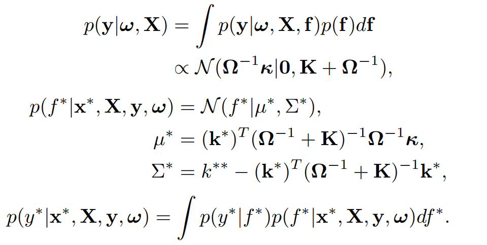
那么对于类别\(t\)的数据，它的似然函数为

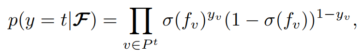
其中\(P^{t}\)是其经过的路径（在代码中通过old_to_new来标注），\(v\)是对应的节点。得到的几个后验分布为

Kernel function

对于一些图片、声音等数据，作者通过DL embedding出一个向量来作为文中的RBF kernel或者Linear kernel等核函数的输入。用户\(c\)对DL参数的优化过程为

\[\begin{align} \nabla\mathcal{L}_c^{ML}(\theta;D_c)&=\sum_v\nabla\log p_\theta(\mathbf{y}_v\vert \mathbf{X}_v)\\ &= \sum_v \frac{\nabla p_\theta(\mathbf{y}_v\vert \mathbf{X}_v)}{p_\theta(\mathbf{y}_v\vert \mathbf{X}_v)}\\ &= \sum_v \frac{\nabla \int_{\omega} p_\theta(\mathbf{y}_v, \omega\vert \mathbf{X}_v)\,d\omega}{p_\theta(\mathbf{y}_v\vert \mathbf{X}_v)}\\ &= \sum_v \int \frac{\nabla p_\theta(\mathbf{y}_v, \omega\vert \mathbf{X}_v)}{p_\theta(\mathbf{y}_v\vert \mathbf{X}_v)}\,d\omega\\ &= \sum_v \int \frac{p_{\theta}(\mathbf{y}_v,\omega\vert \mathbf{X}_v)}{p_\theta(\mathbf{y}_v\vert \mathbf{X}_v)}\nabla\log p_\theta(\mathbf{y}_v,\omega\vert \mathbf{X}_v)\, d\omega\\ &= \sum_v \int p_{\theta}(\omega\vert \mathbf{y}_v, \mathbf{X}_v)\nabla(\log p_\theta(\mathbf{y}_v\vert\omega,\mathbf{X}_v)+\log p(\omega\vert \mathbf{X}_v))\, d\omega\\ &= \sum_v \int p_{\theta}(\omega\vert \mathbf{y}_v, \mathbf{X}_v)\nabla\log p_\theta(\mathbf{y}_v\vert\omega,\mathbf{X}_v)\, d\omega\\ \end{align} \]

Limitied data size

文中是通过广播一组common的数据集来帮助数据量比较小的用户来构建模型的（具体怎么操作看不懂）。

Computational constraint

因为GP里面要求逆，通常是样本数量\(N\)的\(\mathcal{O}(N^3)\)。作者通过上述的common dataset来简化复杂度为\(\mathcal{O}(M^3)\)，其中\(M\)为common dataset的数据集大小。（具体怎么简化的，我感觉就是求逆的时候换了个位置，用common dataset作为训练集）

Summary

厚着脸皮来写个summary吧，

• 作者说要为数据量不足的用户也构建个性化模型，然后就想到了在少样本情况下表现也不错的GP。按作者的话，整个系统学的是一个kernel function前的DL网络，这个网络是所有用户共享的。
• 作者解决limited data size和compuitational constraint的方法都是通过一个common dataset（文中叫做inducing points)，然后把其当作trainning set。怎么说呢，给我的感觉并不是从方法上进行了创新。整个文章的逻辑像是这个样子：GP在样本少的时候表现很好\(\rightarrow\)可以拿来做\(PFL\)；用户数据量小\(\rightarrow\)我给他广播一组数据当训练集还可以解决求逆过程中复杂度高的问题（对数据量大的用户）。所以那我直接广播一批共享的数据，不用GP不就好了。
• 总而言之，作者还是提出了一种PFL的方法。（代码没看懂，各种概率看着也头大，反正我是不会用的）