Decomposition

Decomposition Problem

Introduction

Decomposition is a approach to solving a problem by breaking it up into smaller ones and solving each of smaller ones separately, or sequentially.

If the problem is separable, i.e., the objective is comprised by the sum of functions of sub-vector $x_i$ and each constraint only involve only one variable from one of the sub-vector $x_i$, then each smaller problem involving $x_i$ separately can be easily solved(called trivially parallelizable or block separable). The more interesting problem is that sub-vectors are tangled.

The core idea of decomposition is: using effective methods to solve sub-problems and combining the results in such a way as to solve the larger problem. Two techniques will be introduced in the following.

Primal decomposition

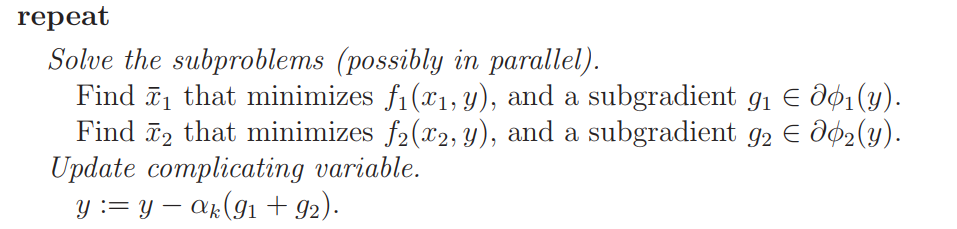
unconstrainted case

$$minf(x)=f_1(x_1,y)+f_2(x_2,y)$$

where $x_1$ and $x_2$ are called private or local variables, $y$ is the complicating or coupling variable which complicates the problem and $x=\{x_1,x_2,y\}$. If $y$ is fixed, the problem is separable and the subproblem is equivalent to find ${\varphi }_1(y)=\underset{x_1}{min}{f}_1(x_1,y)$ and ${\varphi }_2(y)=\underset{x_2}{min}{f}_2(x_2,y)$. The original problem becomes

$$\underset{y}{min}{\varphi }_1(y)+{\varphi }_2(y)$$

which is called master problem.

A decomposition method solve the original problem by a iterative method, such as the subgradient method.

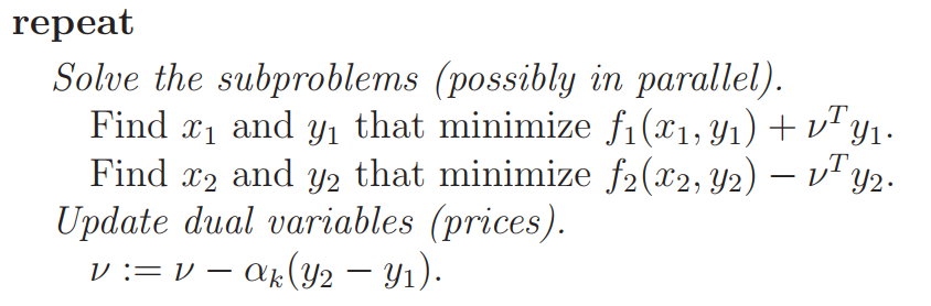
Dual decomposition

consistency constraint

$$\begin{array}{}\text{(1)}& & min{f}_1(x_1,y_1)+f_2(x_2,y_2)\text{(2)}& & \text{s.t.}{y}_1=y_2\end{array}$$

The Lagrangian is

$$L(x_1,x_2,y_1,y_2,v)=f_1(x_1,y_1)+f_2(x_2,y_2)+v^T{y}_1-v^T{y}_2$$

The dual function is

$$g(v)=g_1(v)+g_2(v)$$

where $g_1(v)=\underset{x_1,y_1}{inf}{f}_1(x_1,y_1)+v^T{y}_1=-f_1^{\ast }(0,-v)$, $g_2(v)=\underset{x_2,y_2}{inf}{f}_2(x_2,y_2)-v^T{y}_2=-f_2^{\ast }(0,-v)$

The dual problem is

$$max{g}_1(v)+g_2(v)=min{f}_1^{\ast }(0,-v)+f_2^{\ast }(0,-v)$$

where $g_1(v)$ and $g_2$ can be solved separately, according to the Primal decomposition context.

Decomposition with constraints

$$\begin{array}{}\text{(3)}& min& f_1(x_1)+f_2(x_2)\text{(4)}& \text{s.t.}& x_1\in {\mathcal{C}}_1,x_2\in {\mathcal{C}}_2\text{(5)}& & h_1(x_1)+h_2(x_2)⪯0\end{array}$$

where the last constraint complicates the problem, called complicating constraints.

Primal decomposition

Assigning a fixed amount of resource $t$ to $h_1(x_1)$ and the amount of $h_2(x_2)$ is $-t$, then the original problem can be separable.

$$\begin{array}{}\text{(6)}& min& f_1(x_1)\text{(7)}& \text{s.t.}& x_1\in {\mathcal{C}}_1\text{(8)}& & h_1(x_1)⪯t\end{array}$$

$$\begin{array}{}\text{(9)}& min& f_2(x_2)\text{(10)}& \text{s.t.}& x_2\in {\mathcal{C}}_2\text{(11)}& & h_2(x_2)⪯-t\end{array}$$

Let ${\varphi }_1(t)$ and ${\varphi }_2(t)$ be the optimal value of the problem $\text{6}$ and $\text{9}$, ${\lambda }_1$ and ${\lambda }_2$ denote the optimal dual variable of corresponding subproblem. Then the optimization process is:

1. Solve the subproblem $\text{6}$, to find an optimal $x_1$ and ${\lambda }_1$
2. Solve the subproblem $\text{9}$, to find an optimal $x_2$ and ${\lambda }_2$
3. $t=t-\alpha ({\lambda }_2-{\lambda }_1)$

Dual decomposition

The partial Lagrangian is

$$\begin{array}{}\text{(12)}& L(x_1,x_2,\lambda )& =f_1(x_1)+f_2(x_2)+{\lambda }^T(h_1(x)+h_2(x))\text{(13)}& & =(f_1(x_1)+{\lambda }^T{h}_1(x))+(f_2(x_2)+{\lambda }^T{h}_2(x))\end{array}$$

The problem is the same with $\text{1}$

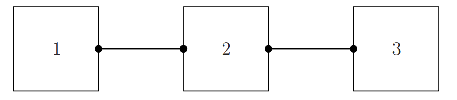
The more complicated decomposition can be represented by a hypergraph or net.

There are three subproblems and each link represent the coupling variable or constraint between the adjoined subproblems.

How primal and dual decomposition work:

• In primal decomposition, each hyperedge or net has a single variable associated with it. Each subproblem is optimized separately, using the public variable values (asserted) on the nets. Each subproblem produces a subgradient associated with each net it is adjacent to. These are combined to update the variable value on the net, hopefully in such a way that convergence to (global) optimality occurs.
• In dual decomposition, each subproblem has its own private copy of the public variables on the nets it is adjacent to, as well as an associated price vector(dual variable ${\lambda }_i$). The subsystems use these prices to optimize their local variables, including the local copies of public variables. The public variables on each net are then compared, and the prices are updated, hopefully in a way that brings the local copies of public variables into consistency (and therefore also optimality).

General framework for decomposition structures

There are $K$ subproblems with private variables $x_i$, public variables $y_i$, public variable $f_i$ and the local feasible set ${\mathcal{C}}_i$. Let $y$ denote the set of all public variables, i.e., $y=(y_1,y_2,\dots ,y_K)$ and $(y{)}_i$ be the $i$-th component. Suppose there are $N$ nets, let $z\in R^N$ be the common value on the nets. Then $y=Ez$, where E is the matrix with

$$E=\{\begin{array}{cc}1& (y{)}_i\text{ is in net j}\\ 0& \text{otherwise}\end{array}$$

The whole problem is

$$\begin{array}{}\text{(14)}& min& \sum _{i=1}^K{f}_i(x_i,y_i)\text{(15)}& \text{s.t.}& (x_i,y_i)\in {\mathcal{C}}_i\text{(16)}& & y_i=E{z}_i\end{array}$$

Primal Decomposition

In primal decomposition, at each iteration we fix the vector z of net variables, and we fix the
public variables as $y_i=E_{i}z$. Each subsystem can (separately) find optimal values for its local variables $x_i$

$$\begin{array}{}\text{(17)}& min& f_i(x_i,y_i)\text{(18)}& \text{s.t.}& (x_i,y_i)\in {\mathcal{C}}_1\end{array}$$

To find a subgradient of $\varphi$, we find $g_i\in \partial {\varphi }_i(y_i)$ . We then have

$$g=\sum _{i=1}^K{E}_i^T{g}_i$$

The entire process is

1. $y_i=E_{i}z,i=1,...,K$
2. Solve subproblems to find optimal $x_i$, and $g_i\in \partial \varphi (y_i),i=1,2\dots ,K$
3. $g=\sum _{i=1}^K{E}_i^T{g}_i$
4. $z=z-{\alpha }_{k}g.$

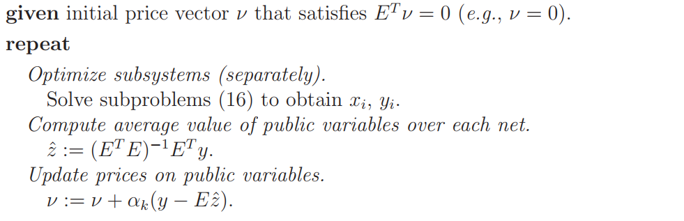
Dual Decomposition

The partial Lagrangian is

$$\begin{array}{}\text{(19)}& L(x,y,z,v)& =\sum _{i=1}^K{f}_i(x_i,y_i)+v^T(y-Ez)\text{(20)}& & =\sum _{i=1}^K{f}_i(x_i,y_i)+v_i^T{y}_i-v^{T}Ez\end{array}$$

the subproblem is

$$\begin{array}{}\text{(21)}& min& f_i(x_i,y_i)+v_i^T{y}_i\text{(22)}& \text{s.t.}& (x_i,y_i)\in {\mathcal{C}}_i\end{array}$$

Let $g_i(v_i)$ be the optimal value of the subproblem and the subgradient of $-g_i$ at $v_i$ is $-y_i$. The dual problem is

$$\begin{array}{}\text{(23)}& max& \sum _{i=1}^K{g}_i(v_i)\text{(24)}& \text{s.t.}& E^{T}v=0\end{array}$$

where the last constraint comes from $\underset{z}{min}L(x,y,z,v)$.

We can solve this dual decomposition master problem using a projected subgradient method. Projection onto the feasible set $\{v|E^{T}v=0\}$, which consists of vectors whose sum over each net is zero. The projection is given by multiplication by $\underset{\text{identity matrix}}{\underbrace{I}}-\underset{\text{average value on the graph}}{\underbrace{E(E^{T}E{)}^{-1}{E}^T}}$, where $E^{T}E=\text{diag}\{d_1,\dots ,d_N\}$, $d_i$ is the degree of the net $i$. $i.e.$, the number of subsystems adjacent to net $i$.