
实用机器学习(快速入门)
前言
因为需要机器学习的助力,所以(浅浅)进修了一下。现在什么东西和AI结合一下感觉就好发文章了;我看了好多学习视频,发现机器学习实际上是数学,并不是常规的去学习代码什么的(虽然代码也很简单),而是去学习原理。这其实并不合我的学习方法,所以我歪门邪道了一下,先实用,再搞原理(这样就比原先快了许多)
这里我比较推荐的唯一的一本书籍是统计学习方法(因为这本书我大概可以看懂,其他方面的书籍都不太适合纯新手)
线性模型(感知机)
直接上代码,通过代码来上手机器学习
import time
import numpy as np
import matplotlib.pyplot as plt
from sklearn.model_selection import train_test_split
from sklearn.linear_model import LinearRegression
from sklearn.metrics import mean_squared_error

# 使用numpy库,随机创建一个数据集
np.random.seed(int(time.time()))
x = 2 * np.random.rand(100, 1)
y = 4 + 3 * x + np.random.rand(100, 1)

# 将数据集进行划分,分为训练集、测试集
X_train, X_test, y_train, y_test = train_test_split(x, y, test_size=0.2,random_state=42)
# 创建线性模型,并开始拟合数据(即训练)
lin_reg = LinearRegression()
lin_reg.fit(X_train, y_train)

print("lin_reg.coef_ ",lin_reg.coef_) # 决策函数的系数
print("lin_reg.intercept_ ", lin_reg.intercept_) # 决策函数的截距
# 开始使用训练好的模型进行预测
y_pred = lin_reg.predict(X_test)

mse = mean_squared_error(y_test, y_pred) # 均方误差回归损失
print("Mean Squared Error: ", mse)

# 可视化
plt.scatter(X_test, y_test)
plt.plot(X_test, lin_reg.predict(X_test), color='red')
plt.title("Linear Regression")
plt.xlabel("x")
plt.ylabel("y")
plt.show()
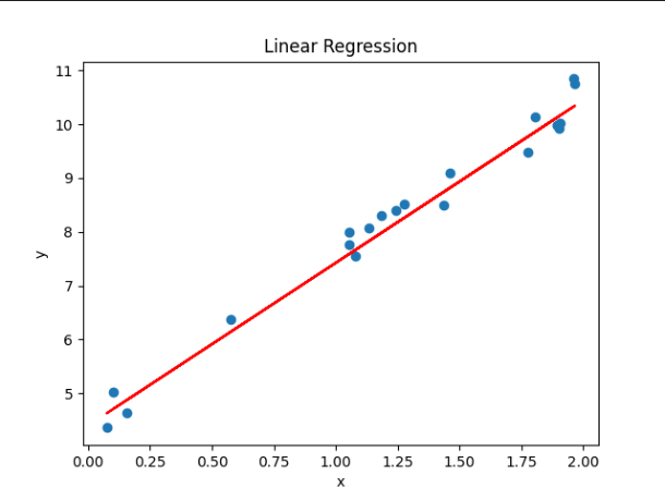
最终展现的如下所示,散点就是实际点。而红线就是我们训练好的模型所拟合好的线,所有的数据都可以在这个线性模型当中进行预测
决策树
决策树其实很好理解,其实就是数据结构当中的普普通通的一棵树,通过判断分支条件最终到达叶子节点来预测结果
import matplotlib.pyplot as plt
from sklearn import tree
from sklearn.datasets import load_iris
import pandas as pd
import numpy as np
from sklearn.model_selection import train_test_split
from sklearn.tree import DecisionTreeClassifier, export_text


# 加载并返回鸢尾花数据集(分类)
iris = load_iris()
# 创建一个表(类似excel),列属性标注为鸢尾花的特征名称
df = pd.DataFrame(iris.data, columns=iris.feature_names)
df['target'] = iris.target # 添加一列为真实值

target = np.unique(iris.target)
target_names = np.unique(iris.target_names)
target_names_dict = dict(zip(target, target_names)) # 迭代生成字典
df['target'] = df['target'].replace(target_names_dict) # 将表中target列数据替换为文字

x = df.drop(columns='target')
y = df['target']
feature_names = x.columns
labels = y.unique()
# 划分训练集、测试集
X_train, X_test, y_train, y_test = train_test_split(x, y, test_size=0.4,random_state=42)
# 决策树最大深度为3
model = DecisionTreeClassifier(max_depth=3, random_state=42) # 初始化模型
model.fit(X_train, y_train) # 训练模型
print(model.score(X_test, y_test)) # 评估模型
print(model.feature_importances_) # 每个特征的权值

r = export_text(model, feature_names=iris.feature_names) # 建立一个文本报告,显示决策树的规则
print(r) # 打印文本报告

plt.figure(figsize=(49,35), facecolor='w') # 创建画布
tree.plot_tree(model, feature_names=feature_names, class_names=labels,
               rounded=True, filled=True, fontsize=60)
plt.show()
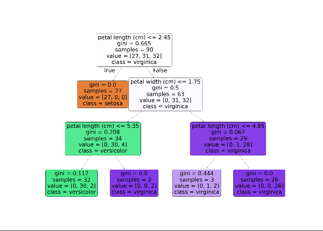
如图所示,这就是我们所训练的决策树模型
神经网络
这里便不同前两个模型,该模型更为复杂了
神经网络是一种模仿生物神经网络结构和功能的计算模型,由大量的人工神经元相互连接而成,具有学习、识别和决策的能力。而我们常常听到的深度学习就是更为复杂的神经网络。
from sklearn import datasets
import matplotlib.pyplot as plt
import numpy as np
import pandas as pd
from sklearn.model_selection import train_test_split
from sklearn.neural_network import MLPClassifier

# 加载数据集
iris = datasets.load_iris()
x = iris.data[:,0:2]
y = iris.target
data = np.hstack((x,y.reshape(y.size,1))) # 进行水平堆叠
# 划分训练集、测试集
x_train,x_test,y_train,y_test = train_test_split(x,y,test_size=0.4,random_state=42)

# 绘制样本点
def plot_samples(ax, x, y):
    n_classes = 3
    plot_colors = "bry"
    for i, color in zip(range(n_classes), plot_colors):
        idx = np.where(y == i)[0]
        ax.scatter(x[idx,0], x[idx,1], c=color, label=iris.target_names[i])
# 绘制等高线
def plot_classifier_predict_meshgrid(ax,clf,x_min,x_max,y_min,y_max):
    plot_step = 0.02
    xx, yy = np.meshgrid(np.arange(x_min, x_max, plot_step),np.arange(y_min, y_max, plot_step))
    z = clf.predict(np.c_[xx.ravel(), yy.ravel()])
    z = z.reshape(xx.shape) # 改变z的维度
    ax.contourf(xx, yy, z) # 绘制等高线


# 多层感知器分类器
classifier = MLPClassifier(activation='logistic', max_iter=10000, hidden_layer_sizes=(30,))
classifier.fit(x_train, y_train) # 训练
train_score = classifier.score(x_train, y_train) # 训练集评估分数
test_score = classifier.score(x_test, y_test) # 测试集评估分数

fig = plt.figure()
ax = fig.add_subplot(1,1,1)
x_min, x_max = x_train[:,0].min() - 1, x_train[:,0].max() + 2
y_min, y_max = x_train[:,1].min() - 1, x_train[:,1].max() + 2
plot_classifier_predict_meshgrid(ax,classifier,x_min, x_max,y_min,y_max) # 绘图(预测的等高线)
plot_samples(ax,x_train,y_train) # 绘图(散点)

ax.legend(loc='best')
ax.set_xlabel(iris.feature_names[0])
ax.set_ylabel(iris.feature_names[1])
ax.set_title("train score:%f;test score:%f"%(train_score,test_score))
plt.show()
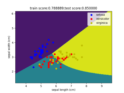
我们经常能听到的所谓调参、炼丹等等,在这里其实便可以有很好的体现,接下来我们简单的调一下参数,来查看不同参数对于准确率的影响有多大?
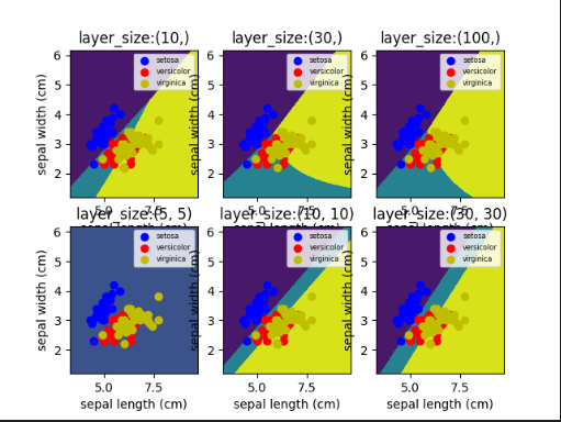
接下来我们首先调整的参数是隐藏层的层数及神经元数这个参数(该参数在神经网络模型当中可谓之最重要的参数之一了)
def for_hidden_layer_size(fig, itx, hidden_layer_sizes):
    # 多层感知器分类器
    classifier = MLPClassifier(activation='logistic', max_iter=10000, hidden_layer_sizes=hidden_layer_sizes)
    classifier.fit(x_train, y_train)  # 训练
    train_score = classifier.score(x_train, y_train)  # 训练集评估分数
    test_score = classifier.score(x_test, y_test)  # 测试集评估分数
    # 开始绘图
    ax = fig.add_subplot(2, 3, itx + 1)
    x_min, x_max = x_train[:, 0].min() - 1, x_train[:, 0].max() + 2
    y_min, y_max = x_train[:, 1].min() - 1, x_train[:, 1].max() + 2
    plot_classifier_predict_meshgrid(ax, classifier, x_min, x_max, y_min, y_max)  # 绘图(预测的等高线)
    plot_samples(ax, x_train, y_train)  # 绘图(散点)
    ax.legend(loc='best', fontsize='xx-small')
    ax.set_xlabel(iris.feature_names[0])
    ax.set_ylabel(iris.feature_names[1])
    ax.set_title("layer_size:%s" % str(hidden_layer_sizes))
    print("layer_size:%s; train score:%.2f; test score:%.2f" % (hidden_layer_sizes, train_score, test_score))

fig = plt.figure()
hidden_layer_sizes = [(10,),(30,),(100,),(5,5),(10,10),(30,30)]
for itx, size in enumerate(hidden_layer_sizes):
    for_hidden_layer_size(fig,itx,size)
plt.show()
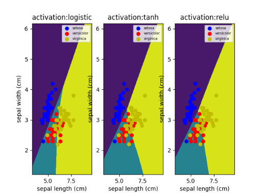
这里我们调整激活函数这个参数,所谓的激活函数就是神经元与神经元之间传递消息的函数。换句话说,A传递给B,那么A是是依靠一个函数来判断传递给B的数据是什么,这个函数就是激活函数。
def for_activation(fig, itx, activation):
    # 多层感知器分类器
    classifier = MLPClassifier(activation=activation, max_iter=10000, hidden_layer_sizes=(30,))
    classifier.fit(x_train, y_train)  # 训练
    train_score = classifier.score(x_train, y_train)  # 训练集评估分数
    test_score = classifier.score(x_test, y_test)  # 测试集评估分数
    # 开始绘图
    ax = fig.add_subplot(1, 3, itx + 1)
    x_min, x_max = x_train[:, 0].min() - 1, x_train[:, 0].max() + 2
    y_min, y_max = x_train[:, 1].min() - 1, x_train[:, 1].max() + 2
    plot_classifier_predict_meshgrid(ax, classifier, x_min, x_max, y_min, y_max)  # 绘图(预测的等高线)
    plot_samples(ax, x_train, y_train)  # 绘图(散点)
    ax.legend(loc='best', fontsize='xx-small')
    ax.set_xlabel(iris.feature_names[0])
    ax.set_ylabel(iris.feature_names[1])
    ax.set_title("activation:%s" % str(activation))
    print("activation:%s; train score:%.2f; test score:%.2f" % (activation, train_score, test_score))

fig = plt.figure()
ativations = ["logistic","tanh","relu"]
for itx, acti in enumerate(ativations):
    for_activation(fig, itx, acti)
plt.show()
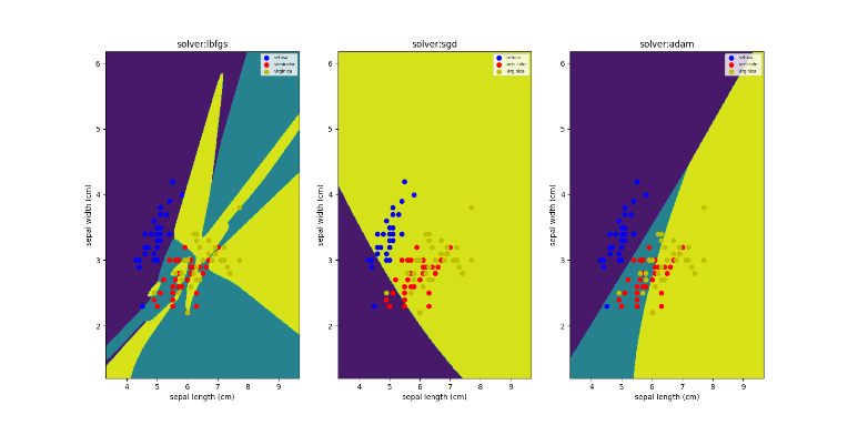
而接下来这个参数,同意重要。solver参数主要是对神经元之间的权重分配的优化算法。也就是A到B之间所占整个体系(层级)的比例是多少
def for_solvers(fig, itx, solver):
    # 多层感知器分类器
    classifier = MLPClassifier(activation='logistic', solver=solver, max_iter=20000, hidden_layer_sizes=(30,))
    classifier.fit(x_train, y_train)  # 训练
    train_score = classifier.score(x_train, y_train)  # 训练集评估分数
    test_score = classifier.score(x_test, y_test)  # 测试集评估分数
    # 开始绘图
    ax = fig.add_subplot(1, 3, itx + 1)
    x_min, x_max = x_train[:, 0].min() - 1, x_train[:, 0].max() + 2
    y_min, y_max = x_train[:, 1].min() - 1, x_train[:, 1].max() + 2
    plot_classifier_predict_meshgrid(ax, classifier, x_min, x_max, y_min, y_max)  # 绘图(预测的等高线)
    plot_samples(ax, x_train, y_train)  # 绘图(散点)
    ax.legend(loc='best', fontsize='xx-small')
    ax.set_xlabel(iris.feature_names[0])
    ax.set_ylabel(iris.feature_names[1])
    ax.set_title("solver:%s" % str(solver))
    print("solver:%s; train score:%.2f; test score:%.2f" % (solver, train_score, test_score))

fig = plt.figure()
fig.set_size_inches(16,8) # 设置图形大小
solvers=["lbfgs","sgd","adam"]
for itx, sol in enumerate(solvers):
    for_solvers(fig, itx, sol)
plt.show()
支持向量机
支持向量机(Support Vector Machine,简称SVM)是一种基于统计学习理论的有监督学习模型,通过寻找特征空间上的最优超平面对样本进行分类或回归。
通俗来说,上面已经学习过了线性模型,线性模型有一个特点就是超平面是直的,无法弯曲。而支持向量机模型的超平面是可以弯曲的。到这里其实引入了一个问题,它是如何弯曲的?
支持向量机引入了一个核函数(所谓的核函数,就是一个将低维数据映射到高维空间当中)将空间升维,在更高的维度当中超平面出现了(高维度的超平面同样是直的,无法弯曲),于此同时将高维度中的超平面映射到低维度时,低维度的(也就是原始空间)超平面就会变的弯曲。
from sklearn import svm
from sklearn.datasets import make_moons
import numpy as np
import matplotlib.pyplot as plt
# 定义绘制决策边界与支持向量的函数
def plot_decision_boundaries(clf, X, y, h=0.02, draw_svm=True, title='Hyperplane'):
# 绘制地图边界
x_min, x_max = X[:, 0].min() - 1, X[:, 0].max() + 1
y_min, y_max = X[:, 1].min() - 1, X[:, 1].max() + 1
xx, yy = np.meshgrid(np.arange(x_min, x_max, h), np.arange(y_min, y_max, h))
# 设置绘图属性
plt.title(title)
plt.xlim(xx.min(), xx.max()) # 限制x轴的显示范围
plt.ylim(yy.min(), yy.max())
plt.xticks(()) # 移除x轴刻度标签
plt.yticks(())
# np.c_用于按列连接数组,ravel用于将多维数组“展平”成一维数组
Z = clf.predict(np.c_[xx.ravel(), yy.ravel()])
Z = Z.reshape(xx.shape)
# 绘制决策边界
plt.contourf(xx, yy, Z, cmap='hot', alpha=0.5)
markers = ('o', 's', '^') # 标记
colors = ('blue', 'red', 'cyan') # 不同颜色用以区分
labels = np.unique(y) # 取标签可能取得的值的类型,此处为0,1
# 绘制数据点
for label in labels:
plt.scatter(X[y == label][:, 0], X[y == label][:, 1], # 散点图
c=colors[label], marker=markers[label])
if draw_svm: # 如果指定绘制支持向量,则绘制支持向量
sv = clf.support_vectors_ # support_vectors_是一个数组,包含所有支持变量
plt.scatter(sv[:, 0], sv[:, 1], c='y', marker='x')
# 生产包含150个样本(月亮形数据集),噪声为0.15
X, y = make_moons(n_samples=150, noise=0.15, random_state=42)
# 初始化不同参数的SVM分类器
# kernel指定算法中使用的内核类型。C为正则化参数,表示对误分类的惩罚程度。gamma定义了单个训练样本的影响达到最大的半径
clf_rbf1 = svm.SVC(kernel='rbf', gamma=0.01, C=1.0)
clf_rbf2 = svm.SVC(kernel='rbf', gamma=5, C=1.0)
clf_rbf3 = svm.SVC(kernel='rbf', gamma=0.01, C=100)
clf_rbf4 = svm.SVC(kernel='rbf', gamma=5, C=100)
clf_rbf5 = svm.SVC(kernel='rbf', gamma=0.01, C=10000)
clf_rbf6 = svm.SVC(kernel='rbf', gamma=5, C=10000)
plt.figure()
clfs = [clf_rbf1, clf_rbf2, clf_rbf3, clf_rbf4, clf_rbf5, clf_rbf6]
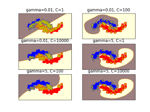
titles = ['gamma=0.01, C=1', 'gamma=0.01, C=100', 'gamma=0.01, C=10000',
'gamma=5, C=1', 'gamma=5, C=100', 'gamma=5, C=10000']
for clf, i in zip(clfs, range(len(clfs))):
clf.fit(X, y) # 训练当前分类器
plt.subplot(3, 2, i+1) # 创建并选择当前子图
plot_decision_boundaries(clf, X, y, title=titles[i])
plt.show()
通过分析结果,发现gamma=0.01,C=1图的决策边界平滑,模型的复杂度较低;如gamma=0.01,C=100图的决策边界同样平滑,但对噪声更加敏感;但是gamma=0.01,C=10000图的C值过大,模型非常复杂,可能存在过拟合的风险;同样的高gamma值也会出现相应的问题,都会带来过拟合的风险
朴素贝叶斯
朴素贝叶斯(Naive Bayes,简称NB)是基于贝叶斯定理与特征条件独立假设的分类方法。其核心思想是利用已知的训练样本集,通过计算待分类样本属于各个类别的概率,并将样本归为概率最大的那个类别
import numpy as np
from matplotlib import pyplot as plt
from matplotlib.colors import ListedColormap
from sklearn.datasets import make_classification, make_moons, make_circles
from sklearn.model_selection import train_test_split
from sklearn.naive_bayes import GaussianNB, MultinomialNB, BernoulliNB, ComplementNB
from sklearn.preprocessing import StandardScaler

# 绘制散点图
def plot_scatter(ax, X_train, y_train, X_test, y_test, array1, array2):
    cm_bright = ListedColormap(['#FF0000', '#0000FF'])
    ax.scatter(X_train[:, 0], X_train[:, 1], c=y_train, cmap=cm_bright, edgecolors='k')
    ax.scatter(X_test[:, 0], X_test[:, 1], c=y_test, cmap=cm_bright, edgecolors='k', alpha=0.6)
    ax.set_xlim(array1.min(), array1.max())
    ax.set_ylim(array2.min(), array2.max())
    ax.set_xticks(())
    ax.set_yticks(())

# 创建模型
def model(clf, datasets, title, typeId=1, typeNum=1, negative=False):
    i = typeId * 2 - 1
    for ds_index, ds in enumerate(datasets):
        X, y = ds
        # 标准化数据集,同时划分训练集和测试集
        X = StandardScaler().fit_transform(X)
        # 如果要求输入是非负值
        if negative:
            min_x = np.min(X[:, 0])
            min_y = np.min(X[:, 1])
            offset = min(abs(min_x), abs(min_y)) + 1  # 加1确保所有值都是正的
            X = X - np.array([min_x, min_y]) + np.array([offset, offset]) # 进行偏移
        # 划分训练集、测试集
        X_train, X_test, y_train, y_test = train_test_split(X, y, test_size=0.4, random_state=42)
        x_min, x_max = X[:, 0].min() - .5, X[:, 0].max() + .5
        y_min, y_max = X[:, 1].min() - .5, X[:, 1].max() + .5
        array1, array2 = np.meshgrid(np.arange(x_min, x_max, 0.2), np.arange(y_min, y_max, 0.2)) # x,y轴坐标
        ax = plt.subplot(len(datasets), 2*typeNum, i) # 子图

        if ds_index == 0:
            ax.set_title('Input Data')
        plot_scatter(ax, X_train, y_train, X_test, y_test, array1, array2)
        # 开始绘制第二幅图
        ax = plt.subplot(len(datasets), 2*typeNum, i + 1)

        clf.fit(X_train, y_train) # 开始训练
        score = clf.score(X_test, y_test) # 评估分数
        Z = clf.predict_proba(np.c_[array1.ravel(), array2.ravel()])[:, 1] # 针对测试向量的概率估计
        Z = Z.reshape(array1.shape)
        ax.contourf(array1, array2, Z, cmap=plt.cm.RdBu, alpha=.8) # 绘制边界
        plot_scatter(ax, X_train, y_train, X_test, y_test, array1, array2)
        if ds_index == 0:
            ax.set_title(title)
        ax.text(array1.max() - .3, array2.min() + .3, ('{:.1f}%'.format(score * 100)), size=15,
                horizontalalignment='right') # 显示测试分数
        i = i + 2 + (typeNum-1)*2

names = ["Multinomial", "Gaussian", "Bernoulli", "Complement"]
# 创建分类器
Classifiers = [MultinomialNB(), GaussianNB(), BernoulliNB(), ComplementNB()]
# 生成数据集。n_features特征总数,n_informative信息特征的数量,n_redundant冗余特征的数量,n_clusters_per_class每个类的簇数
X, y = make_classification(n_features=2, n_informative=2, n_redundant=0, random_state=1, n_clusters_per_class=1)
# 月亮形数据
rng = np.random.RandomState(2)
X += 2 * rng.uniform(size=X.shape)
linearly_separable = (X, y)
# noise加到数据中的高斯噪声的标准偏差,factor内圆和外圆之间的比例因子
datasets = [make_moons(noise=0.3, random_state=0), make_circles(noise=0.2, factor=0.5, random_state=1), linearly_separable]

figure = plt.figure(figsize=(15, 10))

# MultinomialNB与ComplementNB在训练时要求输入数据 X 中的所有特征值都必须是非负的
# 使用四种朴素贝叶斯模型开始训练
for i, clf in enumerate(Classifiers):
    neg = True if i == 0 or i == 3 else False
    model(clf, datasets, names[i], i+1, len(Classifiers), negative=neg)


plt.tight_layout() # 用于自动调整子图参数,使之填充整个图像区域
plt.show()
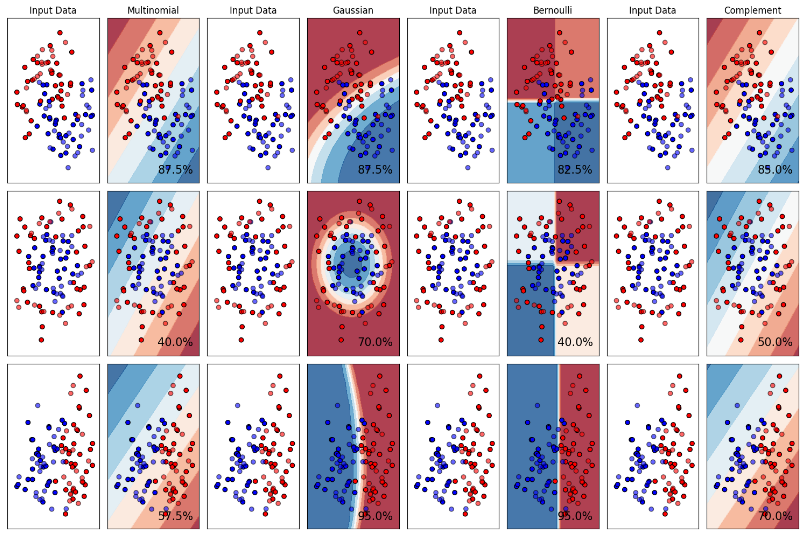
如下图所示,这是四个模型所得出来的结果。我们可以发现在这三种数据分布下,GaussianNB模型最为出色,这其实是因为所给的测试数据较为符合它的应用场景,所以我们在针对不同场景应该选择最合适的模型(侧面说明没有最好的模型,只不过适合不适合而已)
- MultinomialNB(多项式朴素贝叶斯):适用于计数数据,特别是文本数据分类。常用于非常大的数据集
- GaussianNB(高斯朴素贝叶斯):算法简单、易于理解和实现。适用于连续值数据的分类
- BernoulliNB(伯努利朴素贝叶斯):可以处理多类别问题,并且可以处理噪声和不完整的数据。特别适用于二项分布数据(即特征只取0和1两种情况)的分类问题
- ComplementNB(补充朴素贝叶斯):为了修正标准多项式朴素贝叶斯分类器的“严格假设”而设计,特别适合于不平衡的数据集
k-近邻
k近邻(k-Nearest Neighbor,KNN)算法是一种基于实例的学习算法,其核心思想是在特征空间中,如果一个样本附近的k个最近(即特征空间中最邻近)样本的大多数属于某一个类别,则该样本也属于这个类别。这种方法通过测量不同测试样本之间的距离,并寻找最为相近的k个样本来进行分类或回归。
import numpy as np
from matplotlib import pyplot as plt
from matplotlib.colors import ListedColormap
from sklearn import datasets, neighbors
# 设置邻居数
n_neighbors = 15
iris = datasets.load_iris()
X = iris.data[:, :2] # 仅取两个特征
y = iris.target
h = .02 # 步长
cmap_light = ListedColormap(['orange', 'cyan', 'cornflowerblue'])
cmap_bold = ListedColormap(['darkorange', 'c', 'darkblue'])
plt.figure(figsize=(9, 6))
# 遍历两种不同的权重方式:'uniform'(等权重)和'distance'(基于距离的权重)
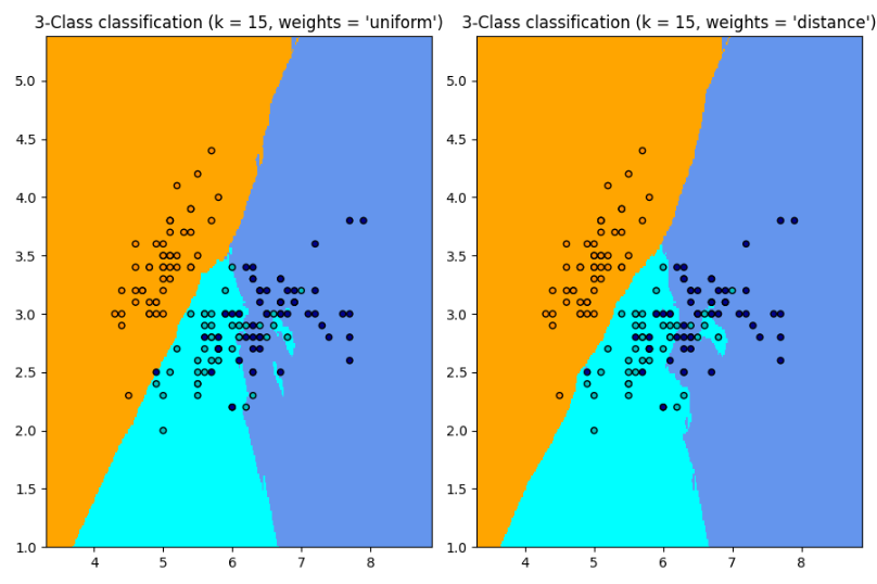
for i, weights in enumerate(['uniform', 'distance']):
# 创建KNN分类器实例,设置邻居数和权重方式
clf = neighbors.KNeighborsClassifier(n_neighbors=n_neighbors, weights=weights)
clf.fit(X, y)
x_min, x_max = X[:, 0].min() - 1, X[:, 0].max() + 1
y_min, y_max = X[:, 1].min() - 1, X[:, 1].max() + 1
xx, yy = np.meshgrid(np.arange(x_min, x_max, h),
np.arange(y_min, y_max, h))
Z = clf.predict(np.c_[xx.ravel(), yy.ravel()])
Z = Z.reshape(xx.shape)
ax = plt.subplot(1, 2, i+1)
# 使用pcolormesh绘制网格的分类颜色
ax.pcolormesh(xx, yy, Z, cmap=cmap_light)
# 绘制原始数据点的散点图,使用不同的颜色表示不同的类别
ax.scatter(X[:, 0], X[:, 1], c=y, cmap=cmap_bold, edgecolors='k', s=20)
ax.set_xlim(xx.min(), xx.max()) # 设置坐标轴的范围
ax.set_ylim(yy.min(), yy.max())
ax.set_title("3-Class classification (k = %i, weights = '%s')"
% (n_neighbors, weights))
plt.tight_layout()
plt.show()
我们首先使用k-近邻分类模型,通过采用iris数据集来进行模拟,发现效果还不错
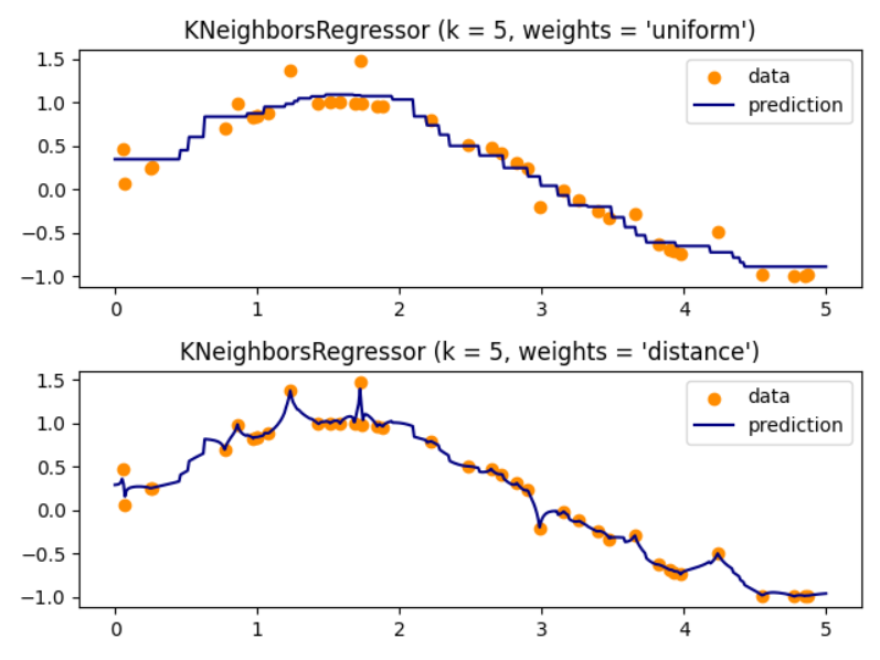
接下来,我们将使用k-近邻回归模型来展示这一算法对于回归问题的效果
import time
import numpy as np
from matplotlib import pyplot as plt
from sklearn import neighbors

np.random.seed(int(time.time()))
X = np.sort(5 * np.random.rand(40, 1), axis=0)
T = np.linspace(0, 5, 500)[:, np.newaxis]
y = np.sin(X).ravel()
y[::5] += 1 * (0.5 - np.random.rand(8))

n_neighbors = 5

for i, weights in enumerate(['uniform', 'distance']):
    knn = neighbors.KNeighborsRegressor(n_neighbors=n_neighbors, weights=weights)
    y_ = knn.fit(X, y).predict(T)

    plt.subplot(2, 1, i+1)
    plt.scatter(X, y, color='darkorange', label='data')
    plt.plot(T, y_, color='navy', label='prediction')
    plt.axis('tight')
    plt.legend()
    plt.title("KNeighborsRegressor (k = %i, weights = '%s')" % (n_neighbors, weights))

plt.tight_layout()
plt.show()
这里我们采用不同的权重函数,发现distance函数对于噪声较为敏感,而uniform函数相对不敏感。这里可以看出权重函数针对同一模型的影响
提升(Boost)算法(集成学习算法)
提升算法(Boosting Algorithms)是一类用于提高机器学习模型预测准确性的集成学习技术。其核心思想是通过结合多个弱学习器(weak learners,即预测准确率略高于随机猜测的模型)来构建一个强学习器(strong learner,即预测准确率较高的模型)
import numpy as np
from matplotlib import pyplot as plt
from sklearn.datasets import make_gaussian_quantiles
from sklearn.ensemble import AdaBoostClassifier
from sklearn.tree import DecisionTreeClassifier

# 生成两组高斯分位数数据
x1, y1 = make_gaussian_quantiles(cov=2.0, n_samples=600, n_features=2,
                                 n_classes=2, random_state=42)
x2, y2 = make_gaussian_quantiles(mean=(3,3), cov=2.0, n_samples=400, n_features=2,
                                 n_classes=2, random_state=42)
# 将两组数据合并
X = np.concatenate((x1, x2)) # 合并特征数据
y = np.concatenate((y1, 1-y2)) # 合并标签数据,注意第二组数据的标签取反以形成分类任务
# 绘制合并后的数据点
plt.figure(figsize=(9, 6))
plt.subplot(1, 2, 1)
plt.scatter(X[:, 0], X[:, 1], marker='o', c=y, s=10)

# DecisionTreeClassifier决策树,max_depth树的最大深度,min_samples_split拆分内部节点所需的最少样本数,min_samples_leaf在叶节点处所需的最小样本数
# 创建并训练AdaBoost模型,estimator建立增强集成的基础估计器(这里是DecisionTreeClassifier)
clf = AdaBoostClassifier(estimator=DecisionTreeClassifier(max_depth=2, min_samples_split=20, min_samples_leaf=5),
                         algorithm="SAMME", n_estimators=200, learning_rate=0.8)
clf.fit(X, y) # 训练模型
# 绘制决策边界
x_min, x_max = X[:, 0].min() - 1, X[:, 0].max() + 1 # 计算x轴的范围
y_min, y_max = X[:, 1].min() - 1, X[:, 1].max() + 1 # 计算y轴的范围
xx, yy = np.meshgrid(np.arange(x_min, x_max, 0.02), np.arange(y_min, y_max, 0.02)) # 生成网格点
Z = clf.predict(np.c_[xx.ravel(), yy.ravel()]) # 对网格点进行预测
Z = Z.reshape(xx.shape) # 重塑预测结果为网格形状

plt.subplot(1, 2, 2)
plt.contourf(xx, yy, Z, alpha=0.7, cmap='coolwarm') # 绘制填充等高线图,显示决策边界
plt.scatter(X[:, 0], X[:, 1], marker='o', c=y, s=10) # 再次绘制数据点,以便与决策边界对比

plt.tight_layout()
plt.show()
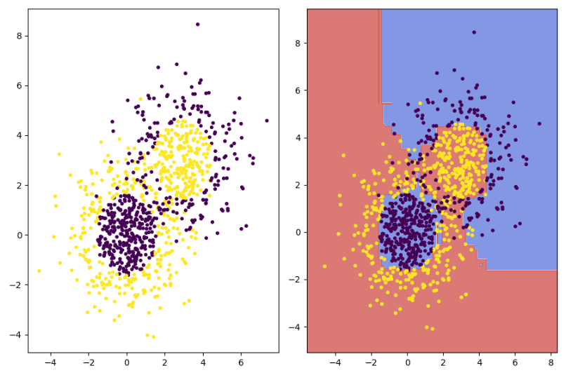
这里我们采用的是AdaBoost模型,同样类似的还有随机森林模型。两者之间最大的不同应该就是串行与并行的特点
- AdaBoost模型:采用Boosting策略。Boosting通过串行训练多个弱学习器,并根据每个弱学习器的表现调整样本的权重,使得后续的学习器更加关注那些在前一轮中被错误分类的样本。
- 随机森林模型:采用Bagging(Bootstrap Aggregating)策略。Bagging通过并行训练多个弱学习器(通常是决策树),并将它们的预测结果进行平均或投票来得到最终预测。
如下图可以看到该模型最后训练出的成果。可以说这个算法所作的一件事情,就是将几个比较弱的专家(也就是垃圾的分类器或者模型)一起凑到一块做决定,来判断最终结果。说白了“三个臭皮匠顶个诸葛亮”(这句话更适用于随机森林模型)
聚类
聚类(Clustering)是机器学习中的一种无监督学习方法,旨在将数据集中的样本划分为若干个类或簇(clusters),使得同一簇内的样本之间相似度较高,而不同簇的样本之间相似度较低。聚类不需要事先知道每个样本的类别标签,而是通过分析样本之间的特征相似性或距离来自动形成簇
from matplotlib import pyplot as plt
from sklearn.cluster import KMeans
from sklearn.datasets import make_blobs
def plot_scatter(X, y, centroid, idx):
color = ["red", "pink", "orange", "gray"]
plt.subplot(1, 3, idx)
for i in range(4):
plt.scatter(X[y == i, 0], X[y == i, 1], color=color[i], marker='o', s=8) # 散点图
plt.scatter(centroid[:, 0], centroid[:, 1], marker='x', s=500, c="black") # 绘制簇中心坐标
def train(n_clusters, X, y, idx):
cluster = KMeans(n_clusters=n_clusters, random_state=0) # K-均值聚类模型
cluster.fit(X) # 训练
centroid = cluster.cluster_centers_ # 簇中心坐标
plot_scatter(X, y, centroid, idx) # 绘制
X, y = make_blobs(n_samples=500, n_features=2, centers=4, random_state=1)
fig = plt.figure(figsize=(15, 6))
# 不同n_clusters参数对于模型的影响
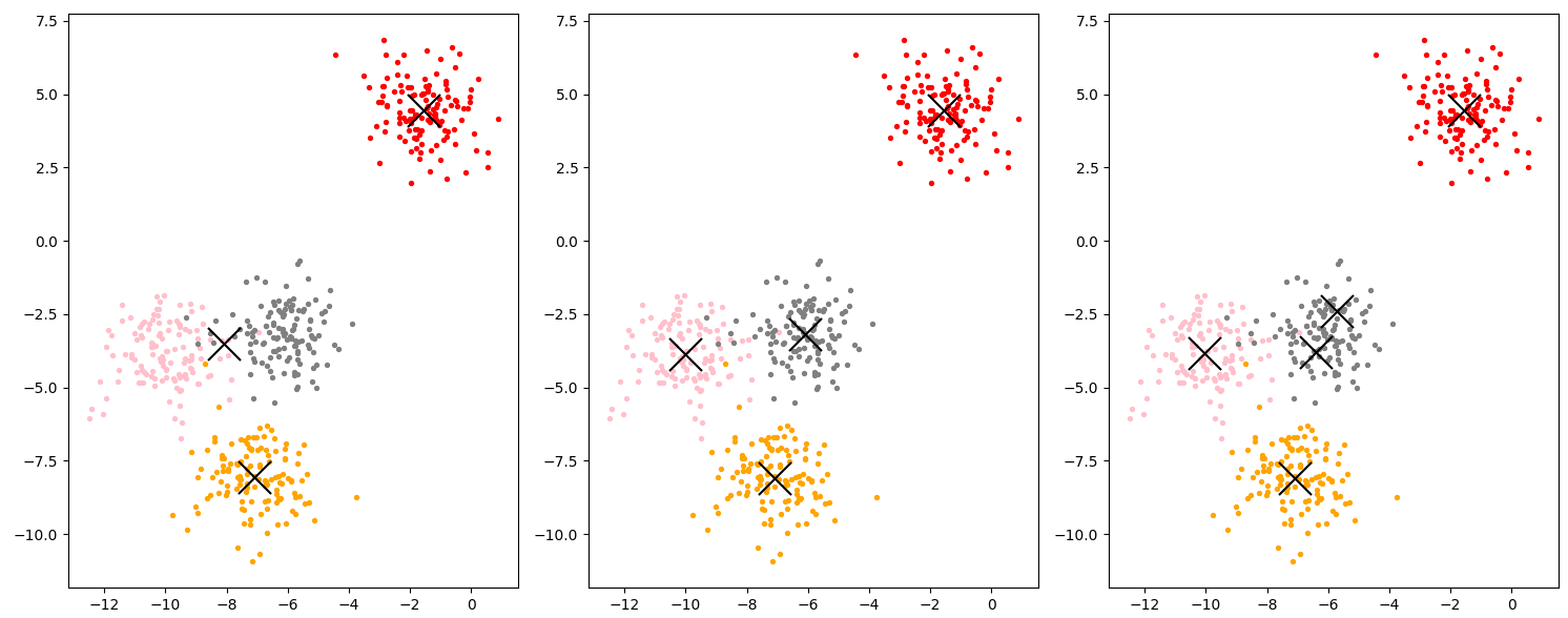
for i in range(1, 4):
train(i+2, X, y, i)
plt.tight_layout()
plt.show()
如下三幅图,不同之处仅在于n_clusters参数的不同(要形成的簇数以及要生成的质心数,也就是说分几类),可以看出中间图最为合适,过少或者过多的簇数都会影响最终的结果及判断


【推荐】国内首个AI IDE,深度理解中文开发场景,立即下载体验Trae
【推荐】编程新体验,更懂你的AI,立即体验豆包MarsCode编程助手
【推荐】抖音旗下AI助手豆包,你的智能百科全书,全免费不限次数
【推荐】轻量又高性能的 SSH 工具 IShell:AI 加持,快人一步
· 周边上新:园子的第一款马克杯温暖上架
· 分享 3 个 .NET 开源的文件压缩处理库,助力快速实现文件压缩解压功能!
· Ollama——大语言模型本地部署的极速利器
· DeepSeek如何颠覆传统软件测试?测试工程师会被淘汰吗?
· 使用C#创建一个MCP客户端