吴恩达深度学习笔记 course2 week3作业

TensorFlow Tutorial

Welcome to this week's programming assignment. Until now, you've always used numpy to build neural networks. Now we will step you through a deep learning framework that will allow you to build neural networks more easily. Machine learning frameworks like TensorFlow, PaddlePaddle, Torch, Caffe, Keras, and many others can speed up your machine learning development significantly. All of these frameworks also have a lot of documentation, which you should feel free to read. In this assignment, you will learn to do the following in TensorFlow:

Initialize variables
Start your own session
Train algorithms
Implement a Neural Network

Programing frameworks can not only shorten your coding time, but sometimes also perform optimizations that speed up your code.

1 - Exploring the Tensorflow Library

To start, you will import the library:

In [1]:

 
import math
import numpy as np
import h5py
import matplotlib.pyplot as plt
import tensorflow as tf
from tensorflow.python.framework import ops
from tf_utils import load_dataset, random_mini_batches, convert_to_one_hot, predict
​
%matplotlib inline
np.random.seed(1)

Now that you have imported the library, we will walk you through its different applications. You will start with an example, where we compute for you the loss of one training example.

l o s s =  (y ̂, y) = (y ̂ (i) - y (i)) 2 (1)

In [3]:

 
y_hat = tf.constant(36, name='y_hat')            # Define y_hat constant. Set to 36.
y = tf.constant(39, name='y')                    # Define y. Set to 39
​
loss = tf.Variable((y - y_hat)**2, name='loss')  # Create a variable for the loss
​
init = tf.global_variables_initializer()         # When init is run later (session.run(init)),
                                                 # the loss variable will be initialized and ready to be computed
with tf.Session() as session:                    # Create a session and print the output
    session.run(init)                            # Initializes the variables
    print(session.run(loss))                     # Prints the loss

Writing and running programs in TensorFlow has the following steps:

Create Tensors (variables) that are not yet executed/evaluated.
Write operations between those Tensors.
Initialize your Tensors.
Create a Session.
Run the Session. This will run the operations you'd written above.

Therefore, when we created a variable for the loss, we simply defined the loss as a function of other quantities, but did not evaluate its value. To evaluate it, we had to run init=tf.global_variables_initializer(). That initialized the loss variable, and in the last line we were finally able to evaluate the value of loss and print its value.

Now let us look at an easy example. Run the cell below:

In [4]:

 
a = tf.constant(2)
b = tf.constant(10)
c = tf.multiply(a,b)
print(c)

Tensor("Mul:0", shape=(), dtype=int32)

As expected, you will not see 20! You got a tensor saying that the result is a tensor that does not have the shape attribute, and is of type "int32". All you did was put in the 'computation graph', but you have not run this computation yet. In order to actually multiply the two numbers, you will have to create a session and run it.

In [5]:

 
sess = tf.Session()
print(sess.run(c))

Great! To summarize, remember to initialize your variables, create a session and run the operations inside the session.

Next, you'll also have to know about placeholders. A placeholder is an object whose value you can specify only later. To specify values for a placeholder, you can pass in values by using a "feed dictionary" (feed_dict variable). Below, we created a placeholder for x. This allows us to pass in a number later when we run the session.

In [6]:

 
# Change the value of x in the feed_dict
​
x = tf.placeholder(tf.int64, name = 'x')
print(sess.run(2 * x, feed_dict = {x: 3}))
sess.close()

When you first defined x you did not have to specify a value for it. A placeholder is simply a variable that you will assign data to only later, when running the session. We say that you feed data to these placeholders when running the session.

Here's what's happening: When you specify the operations needed for a computation, you are telling TensorFlow how to construct a computation graph. The computation graph can have some placeholders whose values you will specify only later. Finally, when you run the session, you are telling TensorFlow to execute the computation graph.

1.1 - Linear function

Lets start this programming exercise by computing the following equation:

Exercise: Compute

X = tf.constant(np.random.randn(3,1), name = "X")

You might find the following functions helpful:

tf.matmul(..., ...) to do a matrix multiplication
tf.add(..., ...) to do an addition
np.random.randn(...) to initialize randomly

In [7]:

 
 
 
 
 

# GRADED FUNCTION: linear_function
​
def linear_function():
    """
    Implements a linear function: 
            Initializes W to be a random tensor of shape (4,3)
            Initializes X to be a random tensor of shape (3,1)
            Initializes b to be a random tensor of shape (4,1)
    Returns: 
    result -- runs the session for Y = WX + b 
    """
    
    np.random.seed(1)
    
    ### START CODE HERE ### (4 lines of code)
    X = tf.constant(np.random.randn(3,1),name="X")
    W = tf.constant(np.random.randn(4,3),name="W")
    b = tf.constant(np.random.randn(4,1),name="b")
    Y = tf.constant(np.random.randn(4,1),name="Y")
    ### END CODE HERE ### 
    
    # Create the session using tf.Session() and run it with sess.run(...) on the variable you want to calculate
    
    ### START CODE HERE ###
    sess = tf.Session()
    result =sess.run(tf.matmul(W,X)+b)
    ### END CODE HERE ### 
    
    # close the session 
    sess.close()
​
    return result
 

In [8]:

 
print( "result = " + str(linear_function()))

result = [[-2.15657382]
 [ 2.95891446]
 [-1.08926781]
 [-0.84538042]]

Expected Output :

result

[[-2.15657382] [ 2.95891446] [-1.08926781] [-0.84538042]]

1.2 - Computing the sigmoid

Great! You just implemented a linear function. Tensorflow offers a variety of commonly used neural network functions like tf.sigmoid and tf.softmax. For this exercise lets compute the sigmoid function of an input.

You will do this exercise using a placeholder variable x. When running the session, you should use the feed dictionary to pass in the input z. In this exercise, you will have to (i) create a placeholder x, (ii) define the operations needed to compute the sigmoid using tf.sigmoid, and then (iii) run the session.

Exercise : Implement the sigmoid function below. You should use the following:

tf.placeholder(tf.float32, name = "...")
tf.sigmoid(...)
sess.run(..., feed_dict = {x: z})

Note that there are two typical ways to create and use sessions in tensorflow:

Method 1:

sess = tf.Session()
# Run the variables initialization (if needed), run the operations
result = sess.run(..., feed_dict = {...})
sess.close() # Close the session

Method 2:

with tf.Session() as sess: 
    # run the variables initialization (if needed), run the operations
    result = sess.run(..., feed_dict = {...})
    # This takes care of closing the session for you :)

In [9]:

 
 
 
 
 

# GRADED FUNCTION: sigmoid
​
def sigmoid(z):
    """
    Computes the sigmoid of z

    Arguments:
    z -- input value, scalar or vector

    Returns: 
    results -- the sigmoid of z
    """
    
    ### START CODE HERE ### ( approx. 4 lines of code)
    # Create a placeholder for x. Name it 'x'.
    x = tf.placeholder(tf.float32,name="x")
​
    # compute sigmoid(x)
    sigmoid = tf.sigmoid(x)
​
    # Create a session, and run it. Please use the method 2 explained above. 
    # You should use a feed_dict to pass z's value to x. 
    with tf.Session() as sess:
        # Run session and call the output "result"
        result = sess.run(sigmoid,feed_dict={x:z})
    sess.close()
    ### END CODE HERE ###
    
    return result
 

In [10]:

 
print ("sigmoid(0) = " + str(sigmoid(0)))
print ("sigmoid(12) = " + str(sigmoid(12)))

sigmoid(0) = 0.5
sigmoid(12) = 0.999994

Expected Output :

sigmoid(0)	0.5
sigmoid(12)	0.999994

To summarize, you how know how to:

Create placeholders
Specify the computation graph corresponding to operations you want to compute
Create the session
Run the session, using a feed dictionary if necessary to specify placeholder variables' values.

1.3 - Computing the Cost

You can also use a built-in function to compute the cost of your neural network. So instead of needing to write code to compute this as a function of

J = - 1 m \sum i = 1 m ( y ( i ) log a [ 2 ] ( i ) + ( 1 -

you can do it in one line of code in tensorflow!

Exercise: Implement the cross entropy loss. The function you will use is:

tf.nn.sigmoid_cross_entropy_with_logits(logits = ..., labels = ...)

Your code should input z, compute the sigmoid (to get a) and then compute the cross entropy cost

- 1 m \sum i = 1 m ( y ( i ) log σ ( z [ 2 ] ( i ) ) + ( 1 -

In [11]:

 
 
 
 
 

# GRADED FUNCTION: cost
​
def cost(logits, labels):
    """
    Computes the cost using the sigmoid cross entropy
    
    Arguments:
    logits -- vector containing z, output of the last linear unit (before the final sigmoid activation)
    labels -- vector of labels y (1 or 0) 

    Note: What we've been calling "z" and "y" in this class are respectively called "logits" and "labels" 
    in the TensorFlow documentation. So logits will feed into z, and labels into y. 
    
    Returns:
    cost -- runs the session of the cost (formula (2))
    """
    
    ### START CODE HERE ### 
    
    # Create the placeholders for "logits" (z) and "labels" (y) (approx. 2 lines)
    z = tf.placeholder(tf.float32,name="logits")
    y = tf.placeholder(tf.float32,name="labels")
    
    # Use the loss function (approx. 1 line)
    cost = tf.nn.sigmoid_cross_entropy_with_logits(logits=z,labels=y)
    
    # Create a session (approx. 1 line). See method 1 above.
    sess = tf.Session()
    
    # Run the session (approx. 1 line).
    cost = sess.run(cost,feed_dict={z:logits ,y:labels})
    
    # Close the session (approx. 1 line). See method 1 above.
    sess.close()
    
    ### END CODE HERE ###
    
    return cost
 

In [12]:

 
logits = sigmoid(np.array([0.2,0.4,0.7,0.9]))
cost = cost(logits, np.array([0,0,1,1]))
print ("cost = " + str(cost))

cost = [ 1.00538719  1.03664088  0.41385433  0.39956614]

Expected Output :

cost

[ 1.00538719 1.03664088 0.41385433 0.39956614]

1.4 - Using One Hot encodings

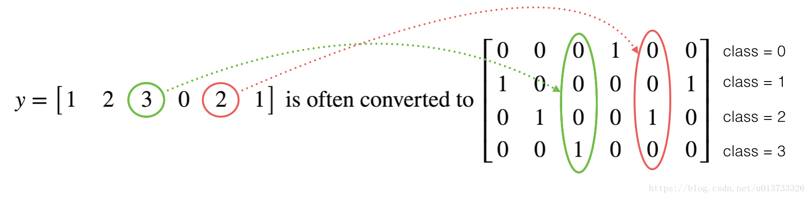
Many times in deep learning you will have a y vector with numbers ranging from 0 to C-1, where C is the number of classes. If C is for example 4, then you might have the following y vector which you will need to convert as follows:

This is called a "one hot" encoding, because in the converted representation exactly one element of each column is "hot" (meaning set to 1). To do this conversion in numpy, you might have to write a few lines of code. In tensorflow, you can use one line of code:

tf.one_hot(labels, depth, axis)

Exercise: Implement the function below to take one vector of labels and the total number of classes

In [13]:

 
 
 
 
 

# GRADED FUNCTION: one_hot_matrix
​
def one_hot_matrix(labels, C):
    """
    Creates a matrix where the i-th row corresponds to the ith class number and the jth column
                     corresponds to the jth training example. So if example j had a label i. Then entry (i,j) 
                     will be 1. 

    Arguments:
    labels -- vector containing the labels 
    C -- number of classes, the depth of the one hot dimension

    Returns: 
    one_hot -- one hot matrix
    """
    
    ### START CODE HERE ###
    
    # Create a tf.constant equal to C (depth), name it 'C'. (approx. 1 line)
    C = tf.constant(C)
    
    # Use tf.one_hot, be careful with the axis (approx. 1 line)
    one_hot_matrix = tf.one_hot(labels,C,axis=0)
    
    # Create the session (approx. 1 line)
    sess =tf.Session()
    
    # Run the session (approx. 1 line)
    one_hot = sess.run(one_hot_matrix)
    
    # Close the session (approx. 1 line). See method 1 above.
    sess.close()
    
    ### END CODE HERE ###
    
    return one_hot
 

In [15]:

 
labels = np.array([1,2,3,0,2,1])
one_hot = one_hot_matrix(labels, C = 4)
print ("one_hot = " + str(one_hot))

one_hot = [[ 0.  0.  0.  1.  0.  0.]
 [ 1.  0.  0.  0.  0.  1.]
 [ 0.  1.  0.  0.  1.  0.]
 [ 0.  0.  1.  0.  0.  0.]]

Expected Output:

one_hot

[[ 0. 0. 0. 1. 0. 0.] [ 1. 0. 0. 0. 0. 1.] [ 0. 1. 0. 0. 1. 0.] [ 0. 0. 1. 0. 0. 0.]]

1.5 - Initialize with zeros and ones

Now you will learn how to initialize a vector of zeros and ones. The function you will be calling is tf.ones(). To initialize with zeros you could use tf.zeros() instead. These functions take in a shape and return an array of dimension shape full of zeros and ones respectively.

Exercise: Implement the function below to take in a shape and to return an array (of the shape's dimension of ones).

tf.ones(shape)

In [16]:

 
# GRADED FUNCTION: ones
​
def ones(shape):
    """
    Creates an array of ones of dimension shape

    Arguments:
    shape -- shape of the array you want to create

    Returns: 
    ones -- array containing only ones
    """
    
    ### START CODE HERE ###
    
    # Create "ones" tensor using tf.ones(...). (approx. 1 line)
    ones = tf.ones(shape)
    
    # Create the session (approx. 1 line)
    sess = tf.Session()
    
    # Run the session to compute 'ones' (approx. 1 line)
    ones = sess.run(ones)
    
    # Close the session (approx. 1 line). See method 1 above.
    sess.close()
    
    ### END CODE HERE ###
    return ones

In [17]:

 
print ("ones = " + str(ones([3])))

ones = [ 1.  1.  1.]

Expected Output:

ones

[ 1. 1. 1.]

2 - Building your first neural network in tensorflow

In this part of the assignment you will build a neural network using tensorflow. Remember that there are two parts to implement a tensorflow model:

Create the computation graph
Run the graph

Let's delve into the problem you'd like to solve!

2.0 - Problem statement: SIGNS Dataset

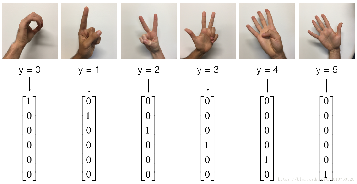
One afternoon, with some friends we decided to teach our computers to decipher sign language. We spent a few hours taking pictures in front of a white wall and came up with the following dataset. It's now your job to build an algorithm that would facilitate communications from a speech-impaired person to someone who doesn't understand sign language.

Training set: 1080 pictures (64 by 64 pixels) of signs representing numbers from 0 to 5 (180 pictures per number).
Test set: 120 pictures (64 by 64 pixels) of signs representing numbers from 0 to 5 (20 pictures per number).

Note that this is a subset of the SIGNS dataset. The complete dataset contains many more signs.

Here are examples for each number, and how an explanation of how we represent the labels. These are the original pictures, before we lowered the image resolutoion to 64 by 64 pixels.

Figure 1: SIGNS dataset

Run the following code to load the dataset.

In [18]:

 
# Loading the dataset
X_train_orig, Y_train_orig, X_test_orig, Y_test_orig, classes = load_dataset()

Change the index below and run the cell to visualize some examples in the dataset.

In [19]:

 
# Example of a picture
index = 0
plt.imshow(X_train_orig[index])
print ("y = " + str(np.squeeze(Y_train_orig[:, index])))

y = 5

As usual you flatten the image dataset, then normalize it by dividing by 255. On top of that, you will convert each label to a one-hot vector as shown in Figure 1. Run the cell below to do so.

In [20]:

 
 
 
 
 

# Flatten the training and test images
X_train_flatten = X_train_orig.reshape(X_train_orig.shape[0], -1).T
X_test_flatten = X_test_orig.reshape(X_test_orig.shape[0], -1).T
# Normalize image vectors
X_train = X_train_flatten/255.
X_test = X_test_flatten/255.
# Convert training and test labels to one hot matrices
Y_train = convert_to_one_hot(Y_train_orig, 6)
Y_test = convert_to_one_hot(Y_test_orig, 6)
​
print ("number of training examples = " + str(X_train.shape[1]))
print ("number of test examples = " + str(X_test.shape[1]))
print ("X_train shape: " + str(X_train.shape))
print ("Y_train shape: " + str(Y_train.shape))
print ("X_test shape: " + str(X_test.shape))
print ("Y_test shape: " + str(Y_test.shape))
 

number of training examples = 1080
number of test examples = 120
X_train shape: (12288, 1080)
Y_train shape: (6, 1080)
X_test shape: (12288, 120)
Y_test shape: (6, 120)

Note that 12288 comes from

Your goal is to build an algorithm capable of recognizing a sign with high accuracy. To do so, you are going to build a tensorflow model that is almost the same as one you have previously built in numpy for cat recognition (but now using a softmax output). It is a great occasion to compare your numpy implementation to the tensorflow one.

The model is LINEAR -> RELU -> LINEAR -> RELU -> LINEAR -> SOFTMAX. The SIGMOID output layer has been converted to a SOFTMAX. A SOFTMAX layer generalizes SIGMOID to when there are more than two classes.

2.1 - Create placeholders

Your first task is to create placeholders for X and Y. This will allow you to later pass your training data in when you run your session.

Exercise: Implement the function below to create the placeholders in tensorflow.

In [21]:

 
 
 
 
 

# GRADED FUNCTION: create_placeholders
​
def create_placeholders(n_x, n_y):
    """
    Creates the placeholders for the tensorflow session.

    Arguments:
    n_x -- scalar, size of an image vector (num_px * num_px = 64 * 64 * 3 = 12288)
    n_y -- scalar, number of classes (from 0 to 5, so -> 6)

    Returns:
    X -- placeholder for the data input, of shape [n_x, None] and dtype "float"
    Y -- placeholder for the input labels, of shape [n_y, None] and dtype "float"

    Tips:
    - You will use None because it let's us be flexible on the number of examples you will for the placeholders.
      In fact, the number of examples during test/train is different.
    """
​
    ### START CODE HERE ### (approx. 2 lines)
    X =tf.placeholder(tf.float32,shape=[n_x,None],name="X")
    Y = tf.placeholder(tf.float32,shape=[n_y,None],name="Y")
    ### END CODE HERE ###
    
    return X, Y
 

In [22]:

 
X, Y = create_placeholders(12288, 6)
print ("X = " + str(X))
print ("Y = " + str(Y))

X = Tensor("X_1:0", shape=(12288, ?), dtype=float32)
Y = Tensor("Y_1:0", shape=(6, ?), dtype=float32)

Expected Output:

X	Tensor("Placeholder_1:0", shape=(12288, ?), dtype=float32) (not necessarily Placeholder_1)
Y	Tensor("Placeholder_2:0", shape=(10, ?), dtype=float32) (not necessarily Placeholder_2)

2.2 - Initializing the parameters

Your second task is to initialize the parameters in tensorflow.

Exercise: Implement the function below to initialize the parameters in tensorflow. You are going use Xavier Initialization for weights and Zero Initialization for biases. The shapes are given below. As an example, to help you, for W1 and b1 you could use:

W1 = tf.get_variable("W1", [25,12288], initializer = tf.contrib.layers.xavier_initializer(seed = 1))
b1 = tf.get_variable("b1", [25,1], initializer = tf.zeros_initializer())

Please use seed = 1 to make sure your results match ours.

In [23]:

 
 
 
 
 

# GRADED FUNCTION: initialize_parameters
​
def initialize_parameters():
    """
    Initializes parameters to build a neural network with tensorflow. The shapes are:
                        W1 : [25, 12288]
                        b1 : [25, 1]
​
                        W2 : [12, 25]
                        b2 : [12, 1]
                        W3 : [6, 12]
                        b3 : [6, 1]

    Returns:
    parameters -- a dictionary of tensors containing W1, b1, W2, b2, W3, b3
    """
    
    tf.set_random_seed(1)                   # so that your "random" numbers match ours
        
    ### START CODE HERE ### (approx. 6 lines of code)
    W1 = tf.get_variable("W1",[25,12288],initializer =tf.contrib.layers.xavier_initializer(seed=1))
    b1 = tf.get_variable("b1",[25,1],initializer =tf.zeros_initializer())
    W2 = tf.get_variable("W2",[12,25],initializer =tf.contrib.layers.xavier_initializer(seed=1))
    b2 = tf.get_variable("b2",[12,1],initializer =tf.zeros_initializer())
    W3 = tf.get_variable("W3",[6,12],initializer =tf.contrib.layers.xavier_initializer(seed=1))
    b3 = tf.get_variable("b3",[6,1],initializer =tf.zeros_initializer())
    ### END CODE HERE ###
​
    parameters = {"W1": W1,
                  "b1": b1,
                  "W2": W2,
                  "b2": b2,
                  "W3": W3,
                  "b3": b3}
    
    return parameters
 

In [24]:

 
tf.reset_default_graph()
with tf.Session() as sess:
    parameters = initialize_parameters()
    print("W1 = " + str(parameters["W1"]))
    print("b1 = " + str(parameters["b1"]))
    print("W2 = " + str(parameters["W2"]))
    print("b2 = " + str(parameters["b2"]))

W1 = <tf.Variable 'W1:0' shape=(25, 12288) dtype=float32_ref>
b1 = <tf.Variable 'b1:0' shape=(25, 1) dtype=float32_ref>
W2 = <tf.Variable 'W2:0' shape=(12, 25) dtype=float32_ref>
b2 = <tf.Variable 'b2:0' shape=(12, 1) dtype=float32_ref>

Expected Output:

W1	< tf.Variable 'W1:0' shape=(25, 12288) dtype=float32_ref >
b1	< tf.Variable 'b1:0' shape=(25, 1) dtype=float32_ref >
W2	< tf.Variable 'W2:0' shape=(12, 25) dtype=float32_ref >
b2	< tf.Variable 'b2:0' shape=(12, 1) dtype=float32_ref >

As expected, the parameters haven't been evaluated yet.

2.3 - Forward propagation in tensorflow

You will now implement the forward propagation module in tensorflow. The function will take in a dictionary of parameters and it will complete the forward pass. The functions you will be using are:

tf.add(...,...) to do an addition
tf.matmul(...,...) to do a matrix multiplication
tf.nn.relu(...) to apply the ReLU activation

Question: Implement the forward pass of the neural network. We commented for you the numpy equivalents so that you can compare the tensorflow implementation to numpy. It is important to note that the forward propagation stops at z3. The reason is that in tensorflow the last linear layer output is given as input to the function computing the loss. Therefore, you don't need a3!

In [41]:

 
 
 
 
 

# GRADED FUNCTION: forward_propagation
​
def forward_propagation(X, parameters):
    """
    Implements the forward propagation for the model: LINEAR -> RELU -> LINEAR -> RELU -> LINEAR -> SOFTMAX

    Arguments:
    X -- input dataset placeholder, of shape (input size, number of examples)
    parameters -- python dictionary containing your parameters "W1", "b1", "W2", "b2", "W3", "b3"
                  the shapes are given in initialize_parameters
​
    Returns:
    Z3 -- the output of the last LINEAR unit
    """
    
    # Retrieve the parameters from the dictionary "parameters" 
    W1 = parameters['W1']
    b1 = parameters['b1']
    W2 = parameters['W2']
    b2 = parameters['b2']
    W3 = parameters['W3']
    b3 = parameters['b3']
    
    ### START CODE HERE ### (approx. 5 lines)              # Numpy Equivalents:
    Z1 = tf.add(tf.matmul(W1,X),b1)                                           # Z1 = np.dot(W1, X) + b1)
    A1 = tf.nn.relu(Z1)                                              # A1 = relu(Z1)
    Z2 = tf.add(tf.matmul(W2,A1),b2)                                         # Z2 = np.dot(W2, a1) + b2
    A2 = tf.nn.relu(Z2)                                              # A2 = relu(Z2)
    Z3 = tf.add(tf.matmul(W3,A2),b3)                                              # Z3 = np.dot(W3,Z2) + b3
    ### END CODE HERE ###
    
    return Z3
 

In [42]:

 
tf.reset_default_graph()
​
with tf.Session() as sess:
    X, Y = create_placeholders(12288, 6)
    parameters = initialize_parameters()
    Z3 = forward_propagation(X, parameters)
    print("Z3 = " + str(Z3))

Z3 = Tensor("Add_2:0", shape=(6, ?), dtype=float32)

Expected Output:

Z3	Tensor("Add_2:0", shape=(6, ?), dtype=float32)

You may have noticed that the forward propagation doesn't output any cache. You will understand why below, when we get to brackpropagation.

2.4 Compute cost

As seen before, it is very easy to compute the cost using:

tf.reduce_mean(tf.nn.softmax_cross_entropy_with_logits(logits = ..., labels = ...))

Question: Implement the cost function below.

It is important to know that the "logits" and "labels" inputs of tf.nn.softmax_cross_entropy_with_logits are expected to be of shape (number of examples, num_classes). We have thus transposed Z3 and Y for you.
Besides, tf.reduce_mean basically does the summation over the examples.

In [43]:

 
 
 
 
 

# GRADED FUNCTION: compute_cost 
​
def compute_cost(Z3, Y):
    """
    Computes the cost

    Arguments:
    Z3 -- output of forward propagation (output of the last LINEAR unit), of shape (6, number of examples)
    Y -- "true" labels vector placeholder, same shape as Z3

    Returns:
    cost - Tensor of the cost function
    """
    
    # to fit the tensorflow requirement for tf.nn.softmax_cross_entropy_with_logits(...,...)
    logits = tf.transpose(Z3)
    labels = tf.transpose(Y)
    
    ### START CODE HERE ### (1 line of code)
    cost = tf.reduce_mean(tf.nn.softmax_cross_entropy_with_logits(logits=logits,labels=labels))
    ### END CODE HERE ###
    
    return cost
 

In [44]:

 
tf.reset_default_graph()
​
with tf.Session() as sess:
    X, Y = create_placeholders(12288, 6)
    parameters = initialize_parameters()
    Z3 = forward_propagation(X, parameters)
    cost = compute_cost(Z3, Y)
    print("cost = " + str(cost))

cost = Tensor("Mean:0", shape=(), dtype=float32)

Expected Output:

cost

Tensor("Mean:0", shape=(), dtype=float32)

2.5 - Backward propagation & parameter updates

This is where you become grateful to programming frameworks. All the backpropagation and the parameters update is taken care of in 1 line of code. It is very easy to incorporate this line in the model.

After you compute the cost function. You will create an "optimizer" object. You have to call this object along with the cost when running the tf.session. When called, it will perform an optimization on the given cost with the chosen method and learning rate.

For instance, for gradient descent the optimizer would be:

optimizer = tf.train.GradientDescentOptimizer(learning_rate = learning_rate).minimize(cost)

To make the optimization you would do:

_ , c = sess.run([optimizer, cost], feed_dict={X: minibatch_X, Y: minibatch_Y})

This computes the backpropagation by passing through the tensorflow graph in the reverse order. From cost to inputs.

Note When coding, we often use _ as a "throwaway" variable to store values that we won't need to use later. Here, _ takes on the evaluated value of optimizer, which we don't need (and c takes the value of the cost variable).

2.6 - Building the model

Now, you will bring it all together!

Exercise: Implement the model. You will be calling the functions you had previously implemented.

In [45]:

 
 
 
 
 

def model(X_train, Y_train, X_test, Y_test, learning_rate = 0.0001,
          num_epochs = 1500, minibatch_size = 32, print_cost = True):
    """
    Implements a three-layer tensorflow neural network: LINEAR->RELU->LINEAR->RELU->LINEAR->SOFTMAX.

    Arguments:
    X_train -- training set, of shape (input size = 12288, number of training examples = 1080)
    Y_train -- test set, of shape (output size = 6, number of training examples = 1080)
    X_test -- training set, of shape (input size = 12288, number of training examples = 120)
    Y_test -- test set, of shape (output size = 6, number of test examples = 120)
    learning_rate -- learning rate of the optimization
    num_epochs -- number of epochs of the optimization loop
    minibatch_size -- size of a minibatch
    print_cost -- True to print the cost every 100 epochs

    Returns:
    parameters -- parameters learnt by the model. They can then be used to predict.
    """
    
    ops.reset_default_graph()                         # to be able to rerun the model without overwriting tf variables
    tf.set_random_seed(1)                             # to keep consistent results
    seed = 3                                          # to keep consistent results
    (n_x, m) = X_train.shape                          # (n_x: input size, m : number of examples in the train set)
    n_y = Y_train.shape[0]                            # n_y : output size
    costs = []                                        # To keep track of the cost
    
    # Create Placeholders of shape (n_x, n_y)
    ### START CODE HERE ### (1 line)
    X, Y = create_placeholders(n_x, n_y)
    ### END CODE HERE ###
​
    # Initialize parameters
    ### START CODE HERE ### (1 line)
    parameters = initialize_parameters()
    ### END CODE HERE ###
    
    # Forward propagation: Build the forward propagation in the tensorflow graph
    ### START CODE HERE ### (1 line)
    Z3 = forward_propagation(X, parameters)
    ### END CODE HERE ###
    
    # Cost function: Add cost function to tensorflow graph
    ### START CODE HERE ### (1 line)
    cost = compute_cost(Z3, Y)
    ### END CODE HERE ###
    
    # Backpropagation: Define the tensorflow optimizer. Use an AdamOptimizer.
    ### START CODE HERE ### (1 line)
    optimizer = tf.train.AdamOptimizer(learning_rate = learning_rate).minimize(cost)
    ### END CODE HERE ###
    
    # Initialize all the variables
    init = tf.global_variables_initializer()
​
    # Start the session to compute the tensorflow graph
    with tf.Session() as sess:
        
        # Run the initialization
        sess.run(init)
        
        # Do the training loop
        for epoch in range(num_epochs):
​
            epoch_cost = 0.                       # Defines a cost related to an epoch
            num_minibatches = int(m / minibatch_size) # number of minibatches of size minibatch_size in the train set
            seed = seed + 1
            minibatches = random_mini_batches(X_train, Y_train, minibatch_size, seed)
​
            for minibatch in minibatches:
​
                # Select a minibatch
                (minibatch_X, minibatch_Y) = minibatch
                
                # IMPORTANT: The line that runs the graph on a minibatch.
                # Run the session to execute the "optimizer" and the "cost", the feedict should contain a minibatch for (X,Y).
                ### START CODE HERE ### (1 line)
                _ , minibatch_cost =sess.run([optimizer,cost],feed_dict={X:minibatch_X,Y:minibatch_Y})
                ### END CODE HERE ###
                
                epoch_cost += minibatch_cost / num_minibatches
​
            # Print the cost every epoch
            if print_cost == True and epoch % 100 == 0:
                print ("Cost after epoch %i: %f" % (epoch, epoch_cost))
            if print_cost == True and epoch % 5 == 0:
                costs.append(epoch_cost)
                
        # plot the cost
        plt.plot(np.squeeze(costs))
        plt.ylabel('cost')
        plt.xlabel('iterations (per tens)')
        plt.title("Learning rate =" + str(learning_rate))
        plt.show()
​
        # lets save the parameters in a variable
        parameters = sess.run(parameters)
        print ("Parameters have been trained!")
​
        # Calculate the correct predictions
        correct_prediction = tf.equal(tf.argmax(Z3), tf.argmax(Y))
​
        # Calculate accuracy on the test set
        accuracy = tf.reduce_mean(tf.cast(correct_prediction, "float"))
​
        print ("Train Accuracy:", accuracy.eval({X: X_train, Y: Y_train}))
        print ("Test Accuracy:", accuracy.eval({X: X_test, Y: Y_test}))
        
        return parameters
 

Run the following cell to train your model! On our machine it takes about 5 minutes. Your "Cost after epoch 100" should be 1.016458. If it's not, don't waste time; interrupt the training by clicking on the square (⬛) in the upper bar of the notebook, and try to correct your code. If it is the correct cost, take a break and come back in 5 minutes!

In [46]:

 
parameters = model(X_train, Y_train, X_test, Y_test)

Cost after epoch 0: 1.855702
Cost after epoch 100: 1.016458
Cost after epoch 200: 0.733102
Cost after epoch 300: 0.572940
Cost after epoch 400: 0.468774
Cost after epoch 500: 0.381021
Cost after epoch 600: 0.313822
Cost after epoch 700: 0.254158
Cost after epoch 800: 0.203829
Cost after epoch 900: 0.166421
Cost after epoch 1000: 0.141486
Cost after epoch 1100: 0.107580
Cost after epoch 1200: 0.086270
Cost after epoch 1300: 0.059371
Cost after epoch 1400: 0.052228

Parameters have been trained!
Train Accuracy: 0.999074
Test Accuracy: 0.716667

Expected Output:

Train Accuracy	0.999074
Test Accuracy	0.716667

Amazing, your algorithm can recognize a sign representing a figure between 0 and 5 with 71.7% accuracy.

Insights:

Your model seems big enough to fit the training set well. However, given the difference between train and test accuracy, you could try to add L2 or dropout regularization to reduce overfitting.
Think about the session as a block of code to train the model. Each time you run the session on a minibatch, it trains the parameters. In total you have run the session a large number of times (1500 epochs) until you obtained well trained parameters.

2.7 - Test with your own image (optional / ungraded exercise)

Congratulations on finishing this assignment. You can now take a picture of your hand and see the output of your model. To do that:

1. Click on "File" in the upper bar of this notebook, then click "Open" to go on your Coursera Hub.
2. Add your image to this Jupyter Notebook's directory, in the "images" folder
3. Write your image's name in the following code
4. Run the code and check if the algorithm is right!

In [47]:

 
 
 
 
 

import scipy
from PIL import Image
from scipy import ndimage
​
## START CODE HERE ## (PUT YOUR IMAGE NAME) 
my_image = "thumbs_up.jpg"
## END CODE HERE ##
​
# We preprocess your image to fit your algorithm.
fname = "images/" + my_image
image = np.array(ndimage.imread(fname, flatten=False))
my_image = scipy.misc.imresize(image, size=(64,64)).reshape((1, 64*64*3)).T
my_image_prediction = predict(my_image, parameters)
​
plt.imshow(image)
print("Your algorithm predicts: y = " + str(np.squeeze(my_image_prediction)))
 

Your algorithm predicts: y = 3

You indeed deserved a "thumbs-up" although as you can see the algorithm seems to classify it incorrectly. The reason is that the training set doesn't contain any "thumbs-up", so the model doesn't know how to deal with it! We call that a "mismatched data distribution" and it is one of the various of the next course on "Structuring Machine Learning Projects".

What you should remember:

Tensorflow is a programming framework used in deep learning
The two main object classes in tensorflow are Tensors and Operators.
When you code in tensorflow you have to take the following steps:
- Create a graph containing Tensors (Variables, Placeholders ...) and Operations (tf.matmul, tf.add, ...)
- Create a session
- Initialize the session
- Run the session to execute the graph
You can execute the graph multiple times as you've seen in model()
The backpropagation and optimization is automatically done when running the session on the "optimizer" object.

中文版摘自:https://blog.csdn.net/u013733326/article/details/79971488

-------------------------------------------------------------------------z中文版--------------------------------------------------------------------------------------------------------------------

TensorFlow 入门

到目前为止，我们一直在使用numpy来自己编写神经网络。现在我们将一步步的使用深度学习的框架来很容易的构建属于自己的神经网络。我们将学习TensorFlow这个框架：

初始化变量
建立一个会话
训练的算法
实现一个神经网络

使用框架编程不仅可以节省你的写代码时间，还可以让你的优化速度更快。

1 - 导入TensorFlow库

开始之前，我们先导入一些库

import numpy as np
import h5py
import matplotlib.pyplot as plt
import tensorflow as tf
from tensorflow.python.framework import ops
import tf_utils
import time

#%matplotlib inline #如果你使用的是jupyter notebook取消注释
np.random.seed(1)

我们现在已经导入了相关的库，我们将引导你完成不同的应用，我们现在看一下下面的计算损失的公式：

l o s s = L (y^, y) = (y^(i) - y (i)) 2 (1)

y_hat = tf.constant(36,name="y_hat")            #定义y_hat为固定值36
y = tf.constant(39,name="y")                    #定义y为固定值39

loss = tf.Variable((y-y_hat)**2,name="loss" )   #为损失函数创建一个变量

init = tf.global_variables_initializer()        #运行之后的初始化(ession.run(init))
                                                #损失变量将被初始化并准备计算
with tf.Session() as session:                   #创建一个session并打印输出
    session.run(init)                           #初始化变量
    print(session.run(loss))                    #打印损失值

执行结果：：

对于Tensorflow的代码实现而言，实现代码的结构如下：

创建Tensorflow变量（此时，尚未直接计算）
实现Tensorflow变量之间的操作定义
初始化Tensorflow变量
创建Session
运行Session，此时，之前编写操作都会在这一步运行。

因此，当我们为损失函数创建一个变量时，我们简单地将损失定义为其他数量的函数，但没有评估它的价值。为了评估它，我们需要运行init=tf.global_variables_initializer()，初始化损失变量，在最后一行，我们最后能够评估损失的值并打印它的值。

现在让我们看一个简单的例子：

a = tf.constant(2)
b = tf.constant(10)
c = tf.multiply(a,b)

print(c)

执行结果：

Tensor("Mul:0", shape=(), dtype=int32)

正如预料中一样，我们并没有看到结果20，不过我们得到了一个Tensor类型的变量，没有维度，数字类型为int32。我们之前所做的一切都只是把这些东西放到了一个“计算图(computation graph)”中，而我们还没有开始运行这个计算图，为了实际计算这两个数字，我们需要创建一个会话并运行它：

sess = tf.Session()

print(sess.run(c))

执行结果：

总结一下，记得初始化变量，然后创建一个session来运行它。
接下来，我们需要了解一下占位符（placeholders）。占位符是一个对象，它的值只能在稍后指定，要指定占位符的值，可以使用一个feed字典（feed_dict变量）来传入，接下来，我们为x创建一个占位符，这将允许我们在稍后运行会话时传入一个数字。

#利用feed_dict来改变x的值

x = tf.placeholder(tf.int64,name="x")
print(sess.run(2 * x,feed_dict={x:3}))
sess.close()

执行结果：

当我们第一次定义x时，我们不必为它指定一个值。占位符只是一个变量，我们会在运行会话时将数据分配给它。

1.1 - 线性函数

让我们通过计算以下等式来开始编程： $Y = W X + b$

X = tf.constant(np.random.randn(3,1), name = "X")

def linear_function():
    """
    实现一个线性功能：
        初始化W，类型为tensor的随机变量，维度为(4,3)
        初始化X，类型为tensor的随机变量，维度为(3,1)
        初始化b，类型为tensor的随机变量，维度为(4,1)
    返回：
        result - 运行了session后的结果，运行的是Y = WX + b 

    """

    np.random.seed(1) #指定随机种子

    X = np.random.randn(3,1)
    W = np.random.randn(4,3)
    b = np.random.randn(4,1)

    Y = tf.add(tf.matmul(W,X),b) #tf.matmul是矩阵乘法
    #Y = tf.matmul(W,X) + b #也可以以写成这样子

    #创建一个session并运行它
    sess = tf.Session()
    result = sess.run(Y)

    #session使用完毕，关闭它
    sess.close()

    return result

我们来测试一下：

print("result = " +  str(linear_function()))

测试结果：

result = [[-2.15657382]
 [ 2.95891446]
 [-1.08926781]
 [-0.84538042]]

1.2 - 计算sigmoid

我们已经实现了线性函数，TensorFlow提供了多种常用的神经网络的函数比如tf.softmax和 tf.sigmoid。
我们将使用占位符变量x，当运行这个session的时候，我们西药使用使用feed字典来输入z，我们将创建占位符变量x，使用tf.sigmoid来定义操作符，最后运行session，我们会用到下面的代码：

tf.placeholder(tf.float32, name = “…”)
tf.sigmoid(…)
sess.run(…, feed_dict = {x: z})

需要注意的是我们可以使用两种方法来创建并使用session

方法一：

sess = tf.Session()
result = sess.run(...,feed_dict = {...})
sess.close()

方法二：

with tf.Session as sess:
    result = sess.run(...,feed_dict = {...})

我们来实现它：

def sigmoid(z):
    """
    实现使用sigmoid函数计算z

    参数：
        z - 输入的值，标量或矢量

    返回：
        result - 用sigmoid计算z的值

    """

    #创建一个占位符x，名字叫“x”
    x = tf.placeholder(tf.float32,name="x")

    #计算sigmoid(z)
    sigmoid = tf.sigmoid(x)

    #创建一个会话，使用方法二
    with tf.Session() as sess:
        result = sess.run(sigmoid,feed_dict={x:z})

    return result

现在我们测试一下：

print ("sigmoid(0) = " + str(sigmoid(0)))
print ("sigmoid(12) = " + str(sigmoid(12)))

测试结果：

sigmoid(0) = 0.5
sigmoid(12) = 0.999994

1.3 - 计算成本

还可以使用内置函数计算神经网络的成本。因此，不需要编写代码来计算成本函数的 $a^{[2] (i)}$

J = - 1 m \sum i = 1 m ( y ( i ) log a [ 2 ] ( i ) + ( 1 -

实现成本函数，需要用到的是：
tf.nn.sigmoid_cross_entropy_with_logits(logits = ..., labels = ...)

你的代码应该输入z，计算sigmoid（得到 a），然后计算交叉熵成本 $J$

1.4 - 使用独热编码（0、1编码）

很多时候在深度学习中 $y$

tf.one_hot(labels,depth,axis)

下面我们要做的是取一个标签矢量和C类总数，返回一个独热编码。

def one_hot_matrix(lables,C):
    """
    创建一个矩阵，其中第i行对应第i个类号，第j列对应第j个训练样本
    所以如果第j个样本对应着第i个标签，那么entry (i,j)将会是1

    参数：
        lables - 标签向量
        C - 分类数

    返回：
        one_hot - 独热矩阵

    """

    #创建一个tf.constant，赋值为C，名字叫C
    C = tf.constant(C,name="C")

    #使用tf.one_hot，注意一下axis
    one_hot_matrix = tf.one_hot(indices=lables , depth=C , axis=0)

    #创建一个session
    sess = tf.Session()

    #运行session
    one_hot = sess.run(one_hot_matrix)

    #关闭session
    sess.close()

    return one_hot

现在我们来测试一下：

labels = np.array([1,2,3,0,2,1])
one_hot = one_hot_matrix(labels,C=4)
print(str(one_hot))

测试结果：

[[ 0.  0.  0.  1.  0.  0.]
 [ 1.  0.  0.  0.  0.  1.]
 [ 0.  1.  0.  0.  1.  0.]
 [ 0.  0.  1.  0.  0.  0.]]

1.5 - 初始化为0和1

现在我们将学习如何用0或者1初始化一个向量，我们要用到tf.ones()和tf.zeros()，给定这些函数一个维度值那么它们将会返回全是1或0的满足条件的向量/矩阵，我们来看看怎样实现它们：

def ones(shape):
    """
    创建一个维度为shape的变量，其值全为1

    参数：
        shape - 你要创建的数组的维度

    返回：
        ones - 只包含1的数组    
    """

    #使用tf.ones()
    ones = tf.ones(shape)

    #创建会话
    sess = tf.Session()

    #运行会话
    ones = sess.run(ones)

    #关闭会话
    sess.close()

    return ones

测试一下：

print ("ones = " + str(ones([3])))

测试结果：

ones = [ 1.  1.  1.]

2 - 使用TensorFlow构建你的第一个神经网络

我们将会使用TensorFlow构建一个神经网络，需要记住的是实现模型需要做以下两个步骤：
1. 创建计算图
2. 运行计算图

我们开始一步步地走一下：

2.0 - 要解决的问题

一天下午，我们和一些朋友决定教我们的电脑破译手语。我们花了几个小时在白色的墙壁前拍照，于是就有了了以下数据集。现在，你的任务是建立一个算法，使有语音障碍的人与不懂手语的人交流。

训练集：有从0到5的数字的1080张图片(64x64像素)，每个数字拥有180张图片。
测试集：有从0到5的数字的120张图片(64x64像素)，每个数字拥有5张图片。

需要注意的是这是完整数据集的一个子集，完整的数据集包含更多的符号。

下面是每个数字的样本，以及我们如何表示标签的解释。这些都是原始图片，我们实际上用的是64 * 64像素的图片。
hands

图 1: 手势符号数据集

首先我们需要加载数据集：

X_train_orig , Y_train_orig , X_test_orig , Y_test_orig , classes = tf_utils.load_dataset()

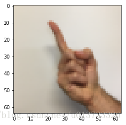
我们可以看一下数据集里面有什么，当然你也可以自己更改一下index的值。

index = 11
plt.imshow(X_train_orig[index])
print("Y = " + str(np.squeeze(Y_train_orig[:,index])))

执行结果：

Y = 1

y=1
和往常一样，我们要对数据集进行扁平化，然后再除以255以归一化数据，除此之外，我们要需要把每个标签转化为独热向量，像上面的图一样。

X_train_flatten = X_train_orig.reshape(X_train_orig.shape[0],-1).T #每一列就是一个样本
X_test_flatten = X_test_orig.reshape(X_test_orig.shape[0],-1).T

#归一化数据
X_train = X_train_flatten / 255
X_test = X_test_flatten / 255

#转换为独热矩阵
Y_train = tf_utils.convert_to_one_hot(Y_train_orig,6)
Y_test = tf_utils.convert_to_one_hot(Y_test_orig,6)

print("训练集样本数 = " + str(X_train.shape[1]))
print("测试集样本数 = " + str(X_test.shape[1]))
print("X_train.shape: " + str(X_train.shape))
print("Y_train.shape: " + str(Y_train.shape))
print("X_test.shape: " + str(X_test.shape))
print("Y_test.shape: " + str(Y_test.shape))

执行结果：

训练集样本数 = 1080
测试集样本数 = 120
X_train.shape: (12288, 1080)
Y_train.shape: (6, 1080)
X_test.shape: (12288, 120)
Y_test.shape: (6, 120)

我们的目标是构建能够高准确度识别符号的算法。要做到这一点，你要建立一个TensorFlow模型，这个模型几乎和你之前在猫识别中使用的numpy一样（但现在使用softmax输出）。要将您的numpy实现与tensorflow实现进行比较的话这是一个很好的机会。

目前的模型是：LINEAR -> RELU -> LINEAR -> RELU -> LINEAR -> SOFTMAX，SIGMOID输出层已经转换为SOFTMAX。当有两个以上的类时，一个SOFTMAX层将SIGMOID一般化。

2.1 - 创建placeholders

我们的第一项任务是为X和Y创建占位符，这将允许我们稍后在运行会话时传递您的训练数据。

def create_placeholders(n_x,n_y):
    """
    为TensorFlow会话创建占位符
    参数：
        n_x - 一个实数，图片向量的大小（64*64*3 = 12288）
        n_y - 一个实数，分类数（从0到5，所以n_y = 6）

    返回：
        X - 一个数据输入的占位符，维度为[n_x, None]，dtype = "float"
        Y - 一个对应输入的标签的占位符，维度为[n_Y,None]，dtype = "float"

    提示：
        使用None，因为它让我们可以灵活处理占位符提供的样本数量。事实上，测试/训练期间的样本数量是不同的。

    """

    X = tf.placeholder(tf.float32, [n_x, None], name="X")
    Y = tf.placeholder(tf.float32, [n_y, None], name="Y")

    return X, Y

测试一下：

X, Y = create_placeholders(12288, 6)
print("X = " + str(X))
print("Y = " + str(Y))

测试结果：

X = Tensor("X:0", shape=(12288, ?), dtype=float32)
Y = Tensor("Y:0", shape=(6, ?), dtype=float32)

2.2 - 初始化参数

初始化tensorflow中的参数，我们将使用Xavier初始化权重和用零来初始化偏差，比如：

W1 = tf.get_variable("W1", [25,12288], initializer = tf.contrib.layers.xavier_initializer(seed = 1))
b1 = tf.get_variable("b1", [25,1], initializer = tf.zeros_initializer())

博主注：tf.Variable() 每次都在创建新对象，对于get_variable()来说，对于已经创建的变量对象，就把那个对象返回，如果没有创建变量对象的话，就创建一个新的。

def initialize_parameters():
    """
    初始化神经网络的参数，参数的维度如下：
        W1 : [25, 12288]
        b1 : [25, 1]
        W2 : [12, 25]
        b2 : [12, 1]
        W3 : [6, 12]
        b3 : [6, 1]

    返回：
        parameters - 包含了W和b的字典


    """

    tf.set_random_seed(1) #指定随机种子

    W1 = tf.get_variable("W1",[25,12288],initializer=tf.contrib.layers.xavier_initializer(seed=1))
    b1 = tf.get_variable("b1",[25,1],initializer=tf.zeros_initializer())
    W2 = tf.get_variable("W2", [12, 25], initializer = tf.contrib.layers.xavier_initializer(seed=1))
    b2 = tf.get_variable("b2", [12, 1], initializer = tf.zeros_initializer())
    W3 = tf.get_variable("W3", [6, 12], initializer = tf.contrib.layers.xavier_initializer(seed=1))
    b3 = tf.get_variable("b3", [6, 1], initializer = tf.zeros_initializer())

    parameters = {"W1": W1,
                  "b1": b1,
                  "W2": W2,
                  "b2": b2,
                  "W3": W3,
                  "b3": b3}

    return parameters

测试一下：

tf.reset_default_graph() #用于清除默认图形堆栈并重置全局默认图形。 

with tf.Session() as sess:
    parameters = initialize_parameters()
    print("W1 = " + str(parameters["W1"]))
    print("b1 = " + str(parameters["b1"]))
    print("W2 = " + str(parameters["W2"]))
    print("b2 = " + str(parameters["b2"]))

测试结果：

W1 = <tf.Variable 'W1:0' shape=(25, 12288) dtype=float32_ref>
b1 = <tf.Variable 'b1:0' shape=(25, 1) dtype=float32_ref>
W2 = <tf.Variable 'W2:0' shape=(12, 25) dtype=float32_ref>
b2 = <tf.Variable 'b2:0' shape=(12, 1) dtype=float32_ref>

正如预期的那样，这些参数只有物理空间，但是还没有被赋值，这是因为没有通过session执行。

2.3 - 前向传播

我们将要在TensorFlow中实现前向传播，该函数将接受一个字典参数并完成前向传播，它会用到以下代码：

tf.add(…) ：加法
tf.matmul(… , …) ：矩阵乘法
tf.nn.relu(…) ：Relu激活函数

我们要实现神经网络的前向传播，我们会拿numpy与TensorFlow实现的神经网络的代码作比较。最重要的是前向传播要在Z3处停止，因为在TensorFlow中最后的线性输出层的输出作为计算损失函数的输入，所以不需要A3.

def forward_propagation(X,parameters):
    """
    实现一个模型的前向传播，模型结构为LINEAR -> RELU -> LINEAR -> RELU -> LINEAR -> SOFTMAX

    参数：
        X - 输入数据的占位符，维度为（输入节点数量，样本数量）
        parameters - 包含了W和b的参数的字典

    返回：
        Z3 - 最后一个LINEAR节点的输出

    """

    W1 = parameters['W1']
    b1 = parameters['b1']
    W2 = parameters['W2']
    b2 = parameters['b2']
    W3 = parameters['W3']
    b3 = parameters['b3']

    Z1 = tf.add(tf.matmul(W1,X),b1)        # Z1 = np.dot(W1, X) + b1
    #Z1 = tf.matmul(W1,X) + b1             #也可以这样写
    A1 = tf.nn.relu(Z1)                    # A1 = relu(Z1)
    Z2 = tf.add(tf.matmul(W2, A1), b2)     # Z2 = np.dot(W2, a1) + b2
    A2 = tf.nn.relu(Z2)                    # A2 = relu(Z2)
    Z3 = tf.add(tf.matmul(W3, A2), b3)     # Z3 = np.dot(W3,Z2) + b3


    return Z3

测试一下：

tf.reset_default_graph() #用于清除默认图形堆栈并重置全局默认图形。 
with tf.Session() as sess:
    X,Y = create_placeholders(12288,6)
    parameters = initialize_parameters()
    Z3 = forward_propagation(X,parameters)
    print("Z3 = " + str(Z3))

测试结果：

Z3 = Tensor("Add_2:0", shape=(6, ?), dtype=float32)

您可能已经注意到前向传播不会输出任何cache，当我们完成反向传播的时候你就会明白了。

2.4 - 计算成本

如前所述，成本很容易计算：

tf.reduce_mean(tf.nn.softmax_cross_entropy_with_logits(logits = ..., labels = ...))

我们现在就来实现计算成本的函数：

def compute_cost(Z3,Y):
    """
    计算成本

    参数：
        Z3 - 前向传播的结果
        Y - 标签，一个占位符，和Z3的维度相同

    返回：
        cost - 成本值


    """
    logits = tf.transpose(Z3) #转置
    labels = tf.transpose(Y)  #转置

    cost = tf.reduce_mean(tf.nn.softmax_cross_entropy_with_logits(logits=logits,labels=labels))

    return cost

测试一下：

tf.reset_default_graph()

with tf.Session() as sess:
    X,Y = create_placeholders(12288,6)
    parameters = initialize_parameters()
    Z3 = forward_propagation(X,parameters)
    cost = compute_cost(Z3,Y)
    print("cost = " + str(cost))

测试结果：

cost = Tensor("Mean:0", shape=(), dtype=float32)

2.5 - 反向传播&更新参数

得益于编程框架，所有反向传播和参数更新都在1行代码中处理。计算成本函数后，将创建一个“optimizer”对象。运行tf.session时，必须将此对象与成本函数一起调用，当被调用时，它将使用所选择的方法和学习速率对给定成本进行优化。

举个例子，对于梯度下降：


optimizer = tf.train.GradientDescentOptimizer(learning_rate = learning_rate).minimize(cost)

要进行优化，应该这样做：


_ , c = sess.run([optimizer,cost],feed_dict={X:mini_batch_X,Y:mini_batch_Y})

编写代码时，我们经常使用 _ 作为一次性变量来存储我们稍后不需要使用的值。这里，_具有我们不需要的优化器的评估值（并且c取值为成本变量的值）。

2.6 - 构建模型

现在我们将实现我们的模型

def model(X_train,Y_train,X_test,Y_test,
        learning_rate=0.0001,num_epochs=1500,minibatch_size=32,
        print_cost=True,is_plot=True):
    """
    实现一个三层的TensorFlow神经网络：LINEAR->RELU->LINEAR->RELU->LINEAR->SOFTMAX

    参数：
        X_train - 训练集，维度为（输入大小（输入节点数量） = 12288, 样本数量 = 1080）
        Y_train - 训练集分类数量，维度为（输出大小(输出节点数量) = 6, 样本数量 = 1080）
        X_test - 测试集，维度为（输入大小（输入节点数量） = 12288, 样本数量 = 120）
        Y_test - 测试集分类数量，维度为（输出大小(输出节点数量) = 6, 样本数量 = 120）
        learning_rate - 学习速率
        num_epochs - 整个训练集的遍历次数
        mini_batch_size - 每个小批量数据集的大小
        print_cost - 是否打印成本，每100代打印一次
        is_plot - 是否绘制曲线图

    返回：
        parameters - 学习后的参数

    """
    ops.reset_default_graph()                #能够重新运行模型而不覆盖tf变量
    tf.set_random_seed(1)
    seed = 3
    (n_x , m)  = X_train.shape               #获取输入节点数量和样本数
    n_y = Y_train.shape[0]                   #获取输出节点数量
    costs = []                               #成本集

    #给X和Y创建placeholder
    X,Y = create_placeholders(n_x,n_y)

    #初始化参数
    parameters = initialize_parameters()

    #前向传播
    Z3 = forward_propagation(X,parameters)

    #计算成本
    cost = compute_cost(Z3,Y)

    #反向传播，使用Adam优化
    optimizer = tf.train.AdamOptimizer(learning_rate=learning_rate).minimize(cost)

    #初始化所有的变量
    init = tf.global_variables_initializer()

    #开始会话并计算
    with tf.Session() as sess:
        #初始化
        sess.run(init)

        #正常训练的循环
        for epoch in range(num_epochs):

            epoch_cost = 0  #每代的成本
            num_minibatches = int(m / minibatch_size)    #minibatch的总数量
            seed = seed + 1
            minibatches = tf_utils.random_mini_batches(X_train,Y_train,minibatch_size,seed)

            for minibatch in minibatches:

                #选择一个minibatch
                (minibatch_X,minibatch_Y) = minibatch

                #数据已经准备好了，开始运行session
                _ , minibatch_cost = sess.run([optimizer,cost],feed_dict={X:minibatch_X,Y:minibatch_Y})

                #计算这个minibatch在这一代中所占的误差
                epoch_cost = epoch_cost + minibatch_cost / num_minibatches

            #记录并打印成本
            ## 记录成本
            if epoch % 5 == 0:
                costs.append(epoch_cost)
                #是否打印：
                if print_cost and epoch % 100 == 0:
                        print("epoch = " + str(epoch) + "    epoch_cost = " + str(epoch_cost))

        #是否绘制图谱
        if is_plot:
            plt.plot(np.squeeze(costs))
            plt.ylabel('cost')
            plt.xlabel('iterations (per tens)')
            plt.title("Learning rate =" + str(learning_rate))
            plt.show()

        #保存学习后的参数
        parameters = sess.run(parameters)
        print("参数已经保存到session。")

        #计算当前的预测结果
        correct_prediction = tf.equal(tf.argmax(Z3),tf.argmax(Y))

        #计算准确率
        accuracy = tf.reduce_mean(tf.cast(correct_prediction,"float"))

        print("训练集的准确率：", accuracy.eval({X: X_train, Y: Y_train}))
        print("测试集的准确率:", accuracy.eval({X: X_test, Y: Y_test}))

        return parameters

我们来正式运行一下模型，请注意，这次的运行时间大约在5-8分钟左右，如果在epoch = 100的时候，你的epoch_cost = 1.01645776539的值和我相差过大，那么你就立即停止，回头检查一下哪里出了问题。

#开始时间
start_time = time.clock()
#开始训练
parameters = model(X_train, Y_train, X_test, Y_test)
#结束时间
end_time = time.clock()
#计算时差
print("CPU的执行时间 = " + str(end_time - start_time) + " 秒" )

运行结果：

epoch = 0    epoch_cost = 1.85570189447
epoch = 100    epoch_cost = 1.01645776539
epoch = 200    epoch_cost = 0.733102379423
epoch = 300    epoch_cost = 0.572938936226
epoch = 400    epoch_cost = 0.468773578604
epoch = 500    epoch_cost = 0.3810211113
epoch = 600    epoch_cost = 0.313826778621
epoch = 700    epoch_cost = 0.254280460603
epoch = 800    epoch_cost = 0.203799342567
epoch = 900    epoch_cost = 0.166511993291
epoch = 1000    epoch_cost = 0.140936921718
epoch = 1100    epoch_cost = 0.107750129745
epoch = 1200    epoch_cost = 0.0862994250475
epoch = 1300    epoch_cost = 0.0609485416137
epoch = 1400    epoch_cost = 0.0509344103436
参数已经保存到session。
训练集的准确率： 0.999074
测试集的准确率: 0.725
CPU的执行时间 = 482.19651398680486 秒

plot

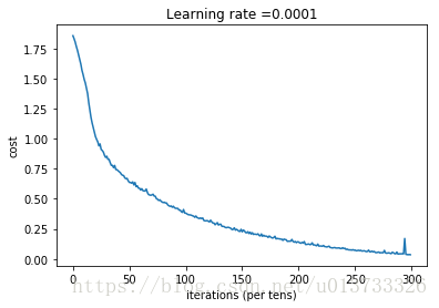
现在，我们的算法已经可以识别0-5的手势符号了，准确率在72.5%。
我们的模型看起来足够大了，可以适应训练集，但是考虑到训练与测试的差异，你也完全可以尝试添加L2或者dropout来减少过拟合。将session视为一组代码来训练模型，在每个minibatch上运行会话时，都会训练我们的参数，总的来说，你已经运行了很多次（1500代），直到你获得训练有素的参数。

2.7 - 测试你自己的图片（选做）

博主自己拍了5张图片，然后裁剪成1：1的样式，再通过格式工厂把很大的图片缩放成64x64的图片，同时把jpg转化为png，因为mpimg只能读取png的图片。

import matplotlib.pyplot as plt # plt 用于显示图片
import matplotlib.image as mpimg # mpimg 用于读取图片
import numpy as np

#这是博主自己拍的图片
my_image1 = "5.png"                                            #定义图片名称
fileName1 = "images/fingers/" + my_image1                      #图片地址
image1 = mpimg.imread(fileName1)                               #读取图片
plt.imshow(image1)                                             #显示图片
my_image1 = image1.reshape(1,64 * 64 * 3).T                    #重构图片
my_image_prediction = tf_utils.predict(my_image1, parameters)  #开始预测
print("预测结果: y = " + str(np.squeeze(my_image_prediction)))

执行结果：

预测结果: y = 5  #预测正确

finger 5

my_image1 = "4.png"

fileName1 = "images/fingers/" + my_image1

image1 = mpimg.imread(fileName1)

plt.imshow(image1)

my_image1 = image1.reshape(1,64 * 64 * 3).T

my_image_prediction = tf_utils.predict(my_image1, parameters)

print("预测结果: y = " + str(np.squeeze(my_image_prediction)))

执行结果：

预测结果: y = 2  #预测错误

my_image1 = "3.png"

fileName1 = "images/fingers/" + my_image1

image1 = mpimg.imread(fileName1)

plt.imshow(image1)

my_image1 = image1.reshape(1,64 * 64 * 3).T

my_image_prediction = tf_utils.predict(my_image1, parameters)

print("预测结果: y = " + str(np.squeeze(my_image_prediction)))

执行结果：

预测结果: y = 2  #预测错误

my_image1 = "2.png"

fileName1 = "images/fingers/" + my_image1

image1 = mpimg.imread(fileName1)

plt.imshow(image1)

my_image1 = image1.reshape(1,64 * 64 * 3).T

my_image_prediction = tf_utils.predict(my_image1, parameters)

print("预测结果: y = " + str(np.squeeze(my_image_prediction)))

执行结果：

预测结果: y = 1  #预测错误

my_image1 = "1.png"

fileName1 = "images/fingers/" + my_image1

image1 = mpimg.imread(fileName1)

plt.imshow(image1)

my_image1 = image1.reshape(1,64 * 64 * 3).T

my_image_prediction = tf_utils.predict(my_image1, parameters)

print("预测结果: y = " + str(np.squeeze(my_image_prediction)))

执行结果：

预测结果: y = 1  #预测正确

posted @ 2018-08-24 08:57 Dar_Alpha 阅读(1325) 评论(0) 编辑收藏举报

会员力量，点亮园子希望

刷新页面返回顶部

吴恩达深度学习笔记 course2 week3作业

TensorFlow Tutorial

1 - Exploring the Tensorflow Library

1.1 - Linear function

1.2 - Computing the sigmoid

1.3 - Computing the Cost

1.4 - Using One Hot encodings

1.5 - Initialize with zeros and ones

2 - Building your first neural network in tensorflow

2.0 - Problem statement: SIGNS Dataset

2.1 - Create placeholders

2.2 - Initializing the parameters

2.3 - Forward propagation in tensorflow

2.4 Compute cost

2.5 - Backward propagation & parameter updates

2.6 - Building the model

2.7 - Test with your own image (optional / ungraded exercise)

TensorFlow 入门

1 - 导入TensorFlow库

1.1 - 线性函数

1.2 - 计算sigmoid

1.3 - 计算成本

1.4 - 使用独热编码（0、1编码）

1.5 - 初始化为0和1

2 - 使用TensorFlow构建你的第一个神经网络

2.0 - 要解决的问题

2.1 - 创建placeholders

2.2 - 初始化参数

2.3 - 前向传播

2.4 - 计算成本

2.5 - 反向传播&更新参数

2.6 - 构建模型

2.7 - 测试你自己的图片（选做）

公告