吴恩达深度学习笔记（四）—— 正则化

有关正则化的详细内容：

吴恩达机器学习笔记（三） —— Regularization正则化

《机器学习实战》学习笔记第五章 —— Logistic回归

 

主要内容：

一.无正则化

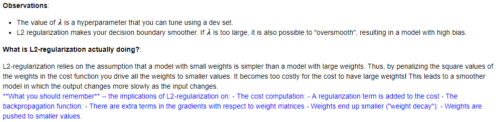
二.L2正则化

三.Dropout正则化

 

 

一.无正则化

深度学习的训练模型如下（可接受“无正则化”、“L2正则化”、“Dropout正则化”三种方式）：

def model(X, Y, learning_rate = 0.3, num_iterations = 30000, print_cost = True, lambd = 0, keep_prob = 1):
    """
    Implements a three-layer neural network: LINEAR->RELU->LINEAR->RELU->LINEAR->SIGMOID.
    
    Arguments:
    X -- input data, of shape (input size, number of examples)
    Y -- true "label" vector (1 for blue dot / 0 for red dot), of shape (output size, number of examples)
    learning_rate -- learning rate of the optimization
    num_iterations -- number of iterations of the optimization loop
    print_cost -- If True, print the cost every 10000 iterations
    lambd -- regularization hyperparameter, scalar
    keep_prob - probability of keeping a neuron active during drop-out, scalar.
    
    Returns:
    parameters -- parameters learned by the model. They can then be used to predict.
    """
        
    grads = {}
    costs = []                            # to keep track of the cost
    m = X.shape[1]                        # number of examples
    layers_dims = [X.shape[0], 20, 3, 1]
    
    # Initialize parameters dictionary.
    parameters = initialize_parameters(layers_dims)

    # Loop (gradient descent)

    for i in range(0, num_iterations):

        # Forward propagation: LINEAR -> RELU -> LINEAR -> RELU -> LINEAR -> SIGMOID.
        if keep_prob == 1:
            a3, cache = forward_propagation(X, parameters)
        elif keep_prob < 1:
            a3, cache = forward_propagation_with_dropout(X, parameters, keep_prob)
        
        # Cost function
        if lambd == 0:
            cost = compute_cost(a3, Y)
        else:
            cost = compute_cost_with_regularization(a3, Y, parameters, lambd)
            
        # Backward propagation.
        assert(lambd==0 or keep_prob==1)    # it is possible to use both L2 regularization and dropout, 
                                            # but this assignment will only explore one at a time
        if lambd == 0 and keep_prob == 1:
            grads = backward_propagation(X, Y, cache)
        elif lambd != 0:
            grads = backward_propagation_with_regularization(X, Y, cache, lambd)
        elif keep_prob < 1:
            grads = backward_propagation_with_dropout(X, Y, cache, keep_prob)
        
        # Update parameters.
        parameters = update_parameters(parameters, grads, learning_rate)
        
        # Print the loss every 10000 iterations
        if print_cost and i % 10000 == 0:
            print("Cost after iteration {}: {}".format(i, cost))
        if print_cost and i % 1000 == 0:
            costs.append(cost)
    
    # plot the cost
    plt.plot(costs)
    plt.ylabel('cost')
    plt.xlabel('iterations (x1,000)')
    plt.title("Learning rate =" + str(learning_rate))
    plt.show()
    
    return parameters

对于无正则化的，直接带入必须参数即可。测试效果如下：

parameters = model(train_X, train_Y)
print ("On the training set:")
predictions_train = predict(train_X, train_Y, parameters)
print ("On the test set:")
predictions_test = predict(test_X, test_Y, parameters)

plt.title("Model without regularization")
axes = plt.gca()
axes.set_xlim([-0.75,0.40])
axes.set_ylim([-0.75,0.65])
plot_decision_boundary(lambda x: predict_dec(parameters, x.T), train_X, train_Y[0])

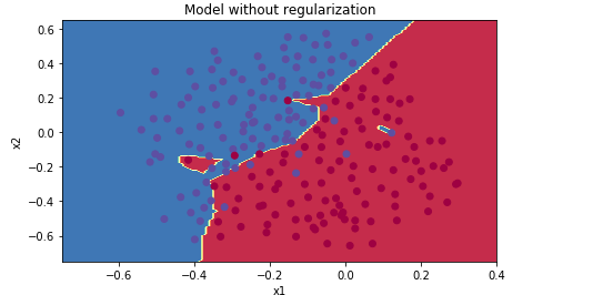
从图像可以看出，无正则化的神经网络，存在过拟合的问题，即便测试准确率已经比较高了。

 

 

二.L2正则化

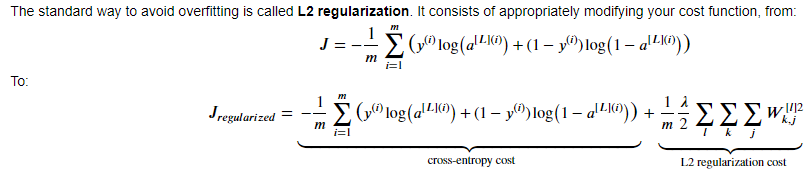
由于使用了正则项，则计算代价的函数和反向传播的函数需要做相应的修改：

代价函数：

# GRADED FUNCTION: compute_cost_with_regularization

def compute_cost_with_regularization(A3, Y, parameters, lambd):
    """
    Implement the cost function with L2 regularization. See formula (2) above.
    
    Arguments:
    A3 -- post-activation, output of forward propagation, of shape (output size, number of examples)
    Y -- "true" labels vector, of shape (output size, number of examples)
    parameters -- python dictionary containing parameters of the model
    
    Returns:
    cost - value of the regularized loss function (formula (2))
    """
    m = Y.shape[1]
    W1 = parameters["W1"]
    W2 = parameters["W2"]
    W3 = parameters["W3"]
    
    cross_entropy_cost = compute_cost(A3, Y) # This gives you the cross-entropy part of the cost
    
    ### START CODE HERE ### (approx. 1 line)
    L2_regularization_cost = lambd/(2*m)*(np.sum(W1**2) + np.sum(W2**2) + np.sum(W3**2))
    ### END CODER HERE ###
    
    cost = cross_entropy_cost + L2_regularization_cost
    
    return cost

反向传播：

# GRADED FUNCTION: backward_propagation_with_regularization

def backward_propagation_with_regularization(X, Y, cache, lambd):
    """
    Implements the backward propagation of our baseline model to which we added an L2 regularization.
    
    Arguments:
    X -- input dataset, of shape (input size, number of examples)
    Y -- "true" labels vector, of shape (output size, number of examples)
    cache -- cache output from forward_propagation()
    lambd -- regularization hyperparameter, scalar
    
    Returns:
    gradients -- A dictionary with the gradients with respect to each parameter, activation and pre-activation variables
    """
    
    m = X.shape[1]
    (Z1, A1, W1, b1, Z2, A2, W2, b2, Z3, A3, W3, b3) = cache
    
    dZ3 = A3 - Y
    
    ### START CODE HERE ### (approx. 1 line)
    dW3 = 1./m * np.dot(dZ3, A2.T) + lambd/m*W3
    ### END CODE HERE ###
    db3 = 1./m * np.sum(dZ3, axis=1, keepdims = True)
    
    dA2 = np.dot(W3.T, dZ3)
    dZ2 = np.multiply(dA2, np.int64(A2 > 0))
    ### START CODE HERE ### (approx. 1 line)
    dW2 = 1./m * np.dot(dZ2, A1.T) +  + lambd/m*W2
    ### END CODE HERE ###
    db2 = 1./m * np.sum(dZ2, axis=1, keepdims = True)
    
    dA1 = np.dot(W2.T, dZ2)
    dZ1 = np.multiply(dA1, np.int64(A1 > 0))
    ### START CODE HERE ### (approx. 1 line)
    dW1 = 1./m * np.dot(dZ1, X.T) +  + lambd/m*W1
    ### END CODE HERE ###
    db1 = 1./m * np.sum(dZ1, axis=1, keepdims = True)
    
    gradients = {"dZ3": dZ3, "dW3": dW3, "db3": db3,"dA2": dA2,
                 "dZ2": dZ2, "dW2": dW2, "db2": db2, "dA1": dA1, 
                 "dZ1": dZ1, "dW1": dW1, "db1": db1}
    
    return gradients

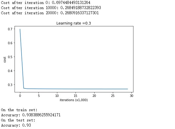
当正则项系数为0.7时，其测试效果如下：

parameters = model(train_X, train_Y, lambd = 0.7)
print ("On the train set:")
predictions_train = predict(train_X, train_Y, parameters)
print ("On the test set:")
predictions_test = predict(test_X, test_Y, parameters)

plt.title("Model with L2-regularization")
axes = plt.gca()
axes.set_xlim([-0.75,0.40])
axes.set_ylim([-0.75,0.65])
plot_decision_boundary(lambda x: predict_dec(parameters, x.T), train_X, train_Y[0])

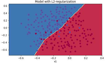
从分类边界可以看出，使用L2正则化的神经网络没有了过拟合的问题，测试准确率也比无正则化的模型高，以此可以证明适当的正则化可以增强模型对数据的泛化能力。

 

 

三.Dropout正则化

（疑问：在前向传播时，A[l]需要除以keep_prob以保持A[l]的取值规模。在发现传播时，根据逆过程的一般思路，dA[l]为什么不是乘上keep_prob，而是又要除以keep_prob呢？）

1.Dropout正则化，并非如L2正则化那样以数学的形式对代价函数引入一个正则项来降低参数的规模，而是一个感性的、较为直观的正则化方式。它的做法是：在每次跌在中，随机关闭一些结点进行前向传播和反向传播、更新参数。每一次迭代所关闭掉的结点可能都不一样。

2.为什么这样随机关闭掉结点的做法可以实现正则化呢？

因为在每次迭代的过程中，实际所训练的模型都是不同的，因为我们用到的只是初始模型的随机子集。由于每个结点在一轮迭代中可能消失，所以一个结点对于其他结点的敏感度降低。这里点自己还没能理解，所以直接看看原话吧：

 

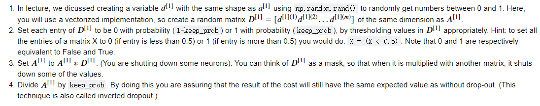
3.前向传播中Dropout的具体步骤如下：

代码实现：

# GRADED FUNCTION: forward_propagation_with_dropout

def forward_propagation_with_dropout(X, parameters, keep_prob = 0.5):
    """
    Implements the forward propagation: LINEAR -> RELU + DROPOUT -> LINEAR -> RELU + DROPOUT -> LINEAR -> SIGMOID.
    
    Arguments:
    X -- input dataset, of shape (2, number of examples)
    parameters -- python dictionary containing your parameters "W1", "b1", "W2", "b2", "W3", "b3":
                    W1 -- weight matrix of shape (20, 2)
                    b1 -- bias vector of shape (20, 1)
                    W2 -- weight matrix of shape (3, 20)
                    b2 -- bias vector of shape (3, 1)
                    W3 -- weight matrix of shape (1, 3)
                    b3 -- bias vector of shape (1, 1)
    keep_prob - probability of keeping a neuron active during drop-out, scalar
    
    Returns:
    A3 -- last activation value, output of the forward propagation, of shape (1,1)
    cache -- tuple, information stored for computing the backward propagation
    """
    
    np.random.seed(1)
    
    # retrieve parameters
    W1 = parameters["W1"]
    b1 = parameters["b1"]
    W2 = parameters["W2"]
    b2 = parameters["b2"]
    W3 = parameters["W3"]
    b3 = parameters["b3"]
    
    # LINEAR -> RELU -> LINEAR -> RELU -> LINEAR -> SIGMOID
    Z1 = np.dot(W1, X) + b1
    A1 = relu(Z1)
    ### START CODE HERE ### (approx. 4 lines)         # Steps 1-4 below correspond to the Steps 1-4 described above. 
    D1 = np.random.rand(A1.shape[0],1)                                         # Step 1: initialize matrix D1 = np.random.rand(..., ...)
    D1 = D1 < keep_prob                                        # Step 2: convert entries of D1 to 0 or 1 (using keep_prob as the threshold)
    A1 = A1 * D1                                         # Step 3: shut down some neurons of A1
    A1 = A1 / keep_prob                                      # Step 4: scale the value of neurons that haven't been shut down
    ### END CODE HERE ###
    Z2 = np.dot(W2, A1) + b2
    A2 = relu(Z2)
    ### START CODE HERE ### (approx. 4 lines)
    D2 = np.random.rand(A2.shape[0],1)                                         # Step 1: initialize matrix D2 = np.random.rand(..., ...)
    D2 = D2 < keep_prob                                              # Step 2: convert entries of D2 to 0 or 1 (using keep_prob as the threshold)
    A2 = A2 * D2                                               # Step 3: shut down some neurons of A2
    A2 = A2 / keep_prob                                                 # Step 4: scale the value of neurons that haven't been shut down
    ### END CODE HERE ###
    Z3 = np.dot(W3, A2) + b3
    A3 = sigmoid(Z3)
    
    cache = (Z1, D1, A1, W1, b1, Z2, D2, A2, W2, b2, Z3, A3, W3, b3)
    
    return A3, cache

 

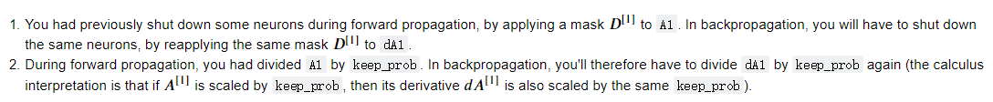
4.反向传播中Dropout的具体步骤如下：

代码实现：

# GRADED FUNCTION: backward_propagation_with_dropout

def backward_propagation_with_dropout(X, Y, cache, keep_prob):
    """
    Implements the backward propagation of our baseline model to which we added dropout.
    
    Arguments:
    X -- input dataset, of shape (2, number of examples)
    Y -- "true" labels vector, of shape (output size, number of examples)
    cache -- cache output from forward_propagation_with_dropout()
    keep_prob - probability of keeping a neuron active during drop-out, scalar
    
    Returns:
    gradients -- A dictionary with the gradients with respect to each parameter, activation and pre-activation variables
    """
    
    m = X.shape[1]
    (Z1, D1, A1, W1, b1, Z2, D2, A2, W2, b2, Z3, A3, W3, b3) = cache
    
    dZ3 = A3 - Y
    dW3 = 1./m * np.dot(dZ3, A2.T)
    db3 = 1./m * np.sum(dZ3, axis=1, keepdims = True)
    dA2 = np.dot(W3.T, dZ3)
    ### START CODE HERE ### (≈ 2 lines of code)
    dA2 = dA2 * D2              # Step 1: Apply mask D2 to shut down the same neurons as during the forward propagation
    dA2 = dA2 / keep_prob              # Step 2: Scale the value of neurons that haven't been shut down
    ### END CODE HERE ###
    dZ2 = np.multiply(dA2, np.int64(A2 > 0))
    dW2 = 1./m * np.dot(dZ2, A1.T)
    db2 = 1./m * np.sum(dZ2, axis=1, keepdims = True)
    
    dA1 = np.dot(W2.T, dZ2)
    ### START CODE HERE ### (≈ 2 lines of code)
    dA1 = dA1 * D1              # Step 1: Apply mask D1 to shut down the same neurons as during the forward propagation
    dA1 = dA1 / keep_prob              # Step 2: Scale the value of neurons that haven't been shut down
    ### END CODE HERE ###
    dZ1 = np.multiply(dA1, np.int64(A1 > 0))
    dW1 = 1./m * np.dot(dZ1, X.T)
    db1 = 1./m * np.sum(dZ1, axis=1, keepdims = True)
    
    gradients = {"dZ3": dZ3, "dW3": dW3, "db3": db3,"dA2": dA2,
                 "dZ2": dZ2, "dW2": dW2, "db2": db2, "dA1": dA1, 
                 "dZ1": dZ1, "dW1": dW1, "db1": db1}
    
    return gradients

 

5.测试效果：

parameters = model(train_X, train_Y, keep_prob = 0.86, learning_rate = 0.3)
print ("On the train set:")
predictions_train = predict(train_X, train_Y, parameters)
print ("On the test set:")
predictions_test = predict(test_X, test_Y, parameters)

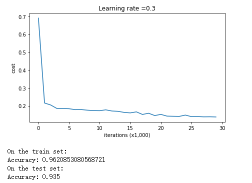
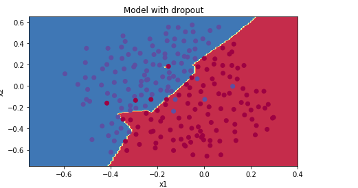
可以看出，三者之中Dropout的测试准确率是最高的，所以说明Dropout正则化是可行的。