对PatchGAN的感知域(receptive_field)理解

for basic discriminator of GANs

判别器用于感知生成器产生的合成图片和ground-truth的差异，并旨在实现区分出fake or real；

同时，判别器的输出也是经过一系列的conv后得到的一个标量值，一般使这个值激活在0~1之间；

但是，这样的结果存在着一些问题：

　　1.输出的结果显然是一个整体图片的加权值，无法体现局部图像的特征，对于精度要求高的的图像迁移等任务比较困难。

for Patch-based discriminator of GANs

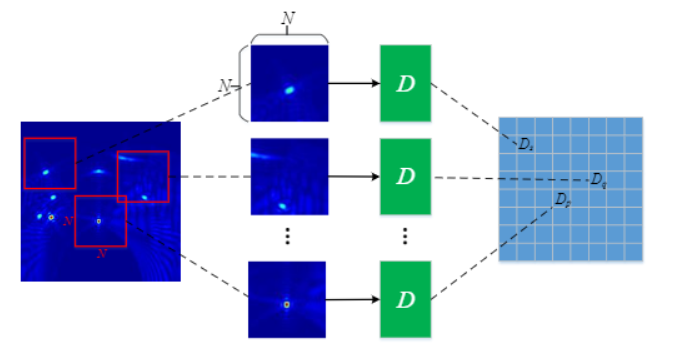
PatchGAN的思路是最后的输出不是一个标量值，而是一个$N*N$的矩阵$X$，其实$X_{ij}$表示patch $ij$是fake or real. 

关键点就是：在$X$上的一个神经元$X_{ij}$可以表示一块输入patch，这个神经元就对这块patch的像素敏感，这块patch 就是 输出$X_{ij}$的感知域(receptive field).

 

1.这样方法 通过每个patch 进行差别的判别， 实现了局部图像特征的提取和表征， 有利于实现更为高分辨率的图像生产；同时， 对最后的 分类特征图进行平均后， 也能够实现相比

2.单标量输出的更为精确的整体差异表示，相当于对整体进行加权求和平均，对于某些特征差异大的局部图像特征， 能够实现比basic D 更为合理的 损失表示。

3.这种机制，将局部图像特征和整体图像特性相融合。

Mathematical：

有个解决办法就是将图像裁剪成多个重叠的patches,分别进行判别器的差异识别，并对得到的结果进行平均，但是这样存在大的运算消耗。

Obviously，卷积神经网络的强大之处在于，它们能以相同的方式独立地处理每个图像块，所以在最后的实际过程中，得到的输出矩阵的每一神经元相当于就是在执行每个patch的单独判断的结果，这样的结果具有高效的运算效果。

The size of receptive field:

堆叠不同层的convnets, 最后输出矩阵的单个神经元的表征的感知域的大小显然不一样；感知域越大，这意味着它应该学习距离更远的对象之间的关系

empirical， 层数越深， 能够感知的patch的尺寸也越大，但是这样会付出更多的计算成本和时间消耗，所以需要通过traceback：

function receptive_field_sizes()


% compute input size from a given output size
f = @(output_size, ksize, stride) (output_size - 1) * stride + ksize;


%% n=1 discriminator

% fix the output size to 1 and derive the receptive field in the input
out = ...
f(f(f(1, 4, 1), ...   % conv2 -> conv3
             4, 1), ...   % conv1 -> conv2
             4, 2);       % input -> conv1

fprintf('n=1 discriminator receptive field size: %d\n', out);


%% n=2 discriminator

% fix the output size to 1 and derive the receptive field in the input
out = ...
f(f(f(f(1, 4, 1), ...   % conv3 -> conv4
             4, 1), ...   % conv2 -> conv3
             4, 2), ...   % conv1 -> conv2
             4, 2);       % input -> conv1

fprintf('n=2 discriminator receptive field size: %d\n', out);


%% n=3 discriminator

% fix the output size to 1 and derive the receptive field in the input
out = ...
f(f(f(f(f(1, 4, 1), ...   % conv4 -> conv5
             4, 1), ...   % conv3 -> conv4
             4, 2), ...   % conv2 -> conv3
             4, 2), ...   % conv1 -> conv2
             4, 2);       % input -> conv1

fprintf('n=3 discriminator receptive field size: %d\n', out);


%% n=4 discriminator

% fix the output size to 1 and derive the receptive field in the input
out = ...
f(f(f(f(f(f(1, 4, 1), ...   % conv5 -> conv6
             4, 1), ...   % conv4 -> conv5
             4, 2), ...   % conv3 -> conv4
             4, 2), ...   % conv2 -> conv3
             4, 2), ...   % conv1 -> conv2
             4, 2);       % input -> conv1

fprintf('n=4 discriminator receptive field size: %d\n', out);


%% n=5 discriminator

% fix the output size to 1 and derive the receptive field in the input
out = ...
f(f(f(f(f(f(f(1, 4, 1), ...   % conv6 -> conv7
             4, 1), ...   % conv5 -> conv6
             4, 2), ...   % conv4 -> conv5
             4, 2), ...   % conv3 -> conv4
             4, 2), ...   % conv2 -> conv3
             4, 2), ...   % conv1 -> conv2
             4, 2);       % input -> conv1

fprintf('n=5 discriminator receptive field size: %d\n', out);

实际模型搭建

显然，是需要堆积多个convnets即可实现PatchGAN的判别器， PatchGAN更多的将它理解为一种机制mechanism，其实整个模型就是一个FCN结构。

对于不同的感知域，肯定在D中表征为有不同的convnet层， torch：

function defineD_n_layers(input_nc, output_nc, ndf, n_layers)
    if n_layers==0 then
        return defineD_pixelGAN(input_nc, output_nc, ndf)
    else
    
        local netD = nn.Sequential()
        
        -- input is (nc) x 256 x 256
        netD:add(nn.SpatialConvolution(input_nc+output_nc, ndf, 4, 4, 2, 2, 1, 1))
        
        module = nn.SpatialConvolution(nInputPlane, nOutputPlane, kW, kH, [dW], [dH], [padW], [padH])
        
        netD:add(nn.LeakyReLU(0.2, true))
        
        local nf_mult = 1
        local nf_mult_prev = 1   
        for n = 1, n_layers-1 do 
            nf_mult_prev = nf_mult
            nf_mult = math.min(2^n,8)
            netD:add(nn.SpatialConvolution(ndf * nf_mult_prev, ndf * nf_mult, 4, 4, 2, 2, 1, 1))
            netD:add(nn.SpatialBatchNormalization(ndf * nf_mult)):add(nn.LeakyReLU(0.2, true))
        end
        
        -- state size: (ndf*M) x N x N
        nf_mult_prev = nf_mult
        nf_mult = math.min(2^n_layers,8)
        netD:add(nn.SpatialConvolution(ndf * nf_mult_prev, ndf * nf_mult, 4, 4, 1, 1, 1, 1))
        netD:add(nn.SpatialBatchNormalization(ndf * nf_mult)):add(nn.LeakyReLU(0.2, true))
        -- state size: (ndf*M*2) x (N-1) x (N-1)
        netD:add(nn.SpatialConvolution(ndf * nf_mult, 1, 4, 4, 1, 1, 1, 1))
        -- state size: 1 x (N-2) x (N-2)
        
        netD:add(nn.Sigmoid())
        -- state size: 1 x (N-2) x (N-2)
        
        return netD
    end
end9

 

一些思考 future works

1.PatchGAN的整个机制的核心在于对 G网络结果的优化，优化了类似U-net的结构(encoder-decoder的架构)，使得低阶信息跨越bottleneck，让更多的低阶信息得以交换，

并让G的训练有如同  Res-block般的平缓梯度，一定程度上减缓了梯度消失， 我们知道Resnet较为好的解决了多层convnet堆叠后的训练困难的问题，其类似于放大器的结构，让训练

更为的有效。

 

2.由于patches的重叠性和局部特征性，对于不同的任务， patches之间的局部特征的相关性肯定存在差异， 所以对于感知域的尺寸确定需要有差异性和动态性，才能实现较为好的性能。

 

3.对于G 来说， 其解码过程其实使用的是微步幅卷积操作或叫做反卷积操作，但是反卷积操作其实对于图像的产生是存在着争议性的，改善和提高这个部分，具有一点的前景， 可以采用

多个的feature map进行重叠作为输入的操作， 得到一个多层特征图， 尝试直接使用一个下采样卷积作为一个生成器。

 

4.对于CGANs 机制的引入， 其实是使得 GAN的训练更加稳定， 进行有约束的执行generative 任务， 进行加 buff的 判别的任务。