GAMES 201 Lecture 2&3 Lagrangian View

Lecture 2&3 Lagrangian View

目录->我的GAMES201学习笔记

• 上节课的几个小问题：

1. 使用 yapf + PEP8 格式化代码

   yapf ... .py
   

2. 输出.gif或是mp4文件(后续会讲)
3. Faster compilation:
   ti.core.toggle_advanced optimization(False) //关闭一些advanced的运算优化以提升速度

Lecture 2 Part

Lagrangian Simulation Approaches

• ——>Mass-Spring Systems and smoothed Particle Hydrodynamics

Mass-Spring Sytems

• 原理：
  
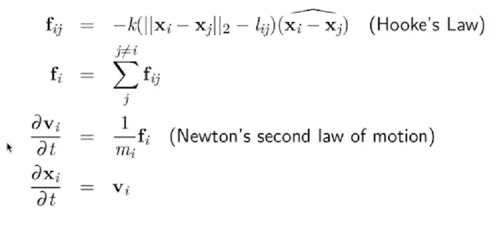
  (胡克定律与牛顿第二定律)

• Time Integration

1. Forward Euler (explicit)
   \(v_{t+1} = v_t+\Delta tm^{-1}f_{t}\)
   \(x_{t+1}=x_t+\Delta tv_t\)
   main characters about explicit methods (like Forward Euler, Symplectic Euler, RK...):
   • Future depends only on past.
   • Easy to implement.
   • Easy to explode : \(\Delta t <= c \sqrt{\frac{m}{k}}\) (c~1) <- 对"硬度"的考量,避免爆炸
   • Bad for stiff materials.
2. Semi-Implicit Euler(a.k.a. symplectic Euler, actually explicit)
   \(v_{t+1}=v_t+\Delta tm^{-1}f_t\)
   \(x_{t+1}=x_t+\Delta tv_{t+1}\)
3. Backward Euler (often with Newton's method, actually implicit)
   main characters about implicit methods (like Backward Euler, middle-point...):
   • Future depends on both future and past.
   • Chicken-egg problem: need to solve a system of linear equations.
   • In general harder to implement.
   • Each step is more expensive but time stpes larger.
   • Nmerical damping and locking.

• Mass-Spring System using implicit method:
  • \(x_{t+1}=x_t+\Delta tv_{t+1}\) ......(1)
  • \(v_{t+1}=v_t+\Delta tM^{-1}f(x_{t+1})\) ......(2)
    Eliminate \(x_{t+1}\) :
  • \(v_{t+1}=v_t+\Delta tM^{-1}f(x_t+\Delta tv_{t+1})\) ......(3)
    Linearize (one step of Newton's method):->使用泰勒展开
  • \(v_{t+1}=v_t+\Delta tM^{-1}[f(x_t)+\frac{\partial f}{\partial x}(x_t)\Delta tv_{t+1}]\) ......(4)
    Clean up(移项):
  • \([I-\Delta t^2M^{-1}\frac{\partial f}{\partial x}(x_t)]v_{t+1}=v_t+\Delta tM^{-1}f(x_t)\) ......(5)
    令
    A=\([I-\Delta t^2M^{-1}\frac{\partial f}{\partial x}(x_t)]\)
    b=\(v_t+\Delta tM^{-1}f(x_t)\)
    得到:
    \(Av_{t+1}=b\) (-> a system of linear equations)
    Solve it ! :
    • Jacobi/Gauss-Seidel iterations (easy to implement)
    • Conjugate gradients (共轭梯度法 以后会讲)
      补充内容：Jacobi迭代法以及实现代码
• \([I-\beta \Delta t^2M^{-1}\frac{\partial f}{\partial x}(x_t)]v_{t+1}=v_t+\Delta tM^{-1}f(x_t)\)
  • \(\beta =0\) -> Forward / Semi-implicit Euler
  • \(\beta =\frac{1}{2}\) -> Middle-point (implicit)
  • \(\beta = 1\) -> Backward Euler(implicit)
• What if we have millions of mass point and springs?
  • Sparse matrices
  • Conjugate gradients
  • Preconditioning
  • Use position-based dynamics
    A different (yet much faster) approach:
    Fast mass_spring system
    ——————————————Lecture 2 施工中————————————————

Lecture 3 Basics of deformation, elasticity & finite elements

Deformation & Elasticity

• Deformation map \(\phi\) : a (vector to vector) function that relates rest material position and deformed material position. (将rest状态的位置映射到deformed状态的函数)
  • \(x_{deformed}=\phi(x_{rest})\)
• Deformation gradient F :
  • F:=\(\frac{\partial x_{deformed}}{\partial x_{rest}}\)
    ※：Deformed gradients are translational invariant,\(\phi_1=\phi(x_{rest})\) and \(\phi_2=\phi(x_{rest})+c\) have the same deformation gradient.
• Deform/rest volume ratio J=det(F) -> (J=\(\frac{Deform Volume}{Rest Volume}\))
• Hyperelastic materials:
  materials whose stress-strain relationship is defined by a strain energy density function.
  (单位体积势能密度)
  • \(\psi=\psi(F)\)
  • Intutive understanding:
    • \(\psi\) is a potential function that penalizes deformation.
    • "Stress"(应力):the material's internal elastic forces.
    • "Strain"(应变):just replace it with deformation gradients F for now.
  • ※Be careful: We use \(\psi\) as the strain energy density function and \(\phi\) as the deformation map. They are completely different.
• Stress tensor. -> 二阶张量.(3x3矩阵)
  • Stress stands for internal forces that infinitesimal material components exert on their neighborhood.
  • The First Piola-Kirchhoff stress tensor (PK1):
    \(P(F)=\frac{\partial \psi(F)}{\partial F}\)
  • Kirchhoff stress:\(\tau\)
  • Cauchy stress tensor: \(\sigma\) (symmetirc, because of conservation of angular momentum).
    Relationship:
    • \(\tau = J\sigma=PF^T\)
    • \(P=J\sigma F^{-T}\)
      (J compensates for material compression expansion,
      \(F^{-T}\) compensates for material deformation.)
    • Traction: \(t = \sigma ^Tn\)
• Elastic moduli (isotropic materials)
  • Young's modulus \(E=\frac{\sigma }{\epsilon }\)
  • Bulk modulus \(K=-V\frac{\mathrm{d}p}{\mathrm{d}V}\) ->常用于可压缩液体
  • Poisson's ratio \(v\in[0.0 , 0.5)\) ->横向正应变与轴向正应变比值
    （Auxetics have negative Poissson's ratio）
• Lamé Parameters:
  • Lamé's first parameter \(\mu\)
  • Lamé's second parameter \(\lambda\) (a.k.a. shear modulus, denot by G)
  • Useful conversion formula:
    • \(K=\frac{E}{3(1-2v)}\)

————————看完太极图形课后再来更新————————————
待补充内容：太极图形课

课后阅读材料：

• Lecture 2 :

• Lecture 3 :