
第7章 PCA与梯度上升法
7-1 什么是PCA


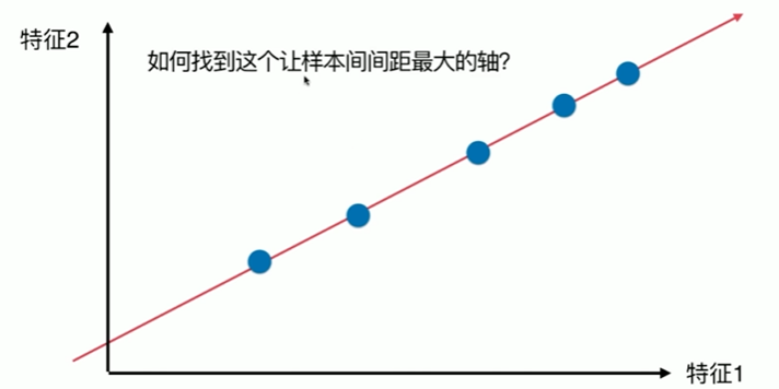
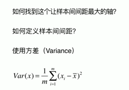
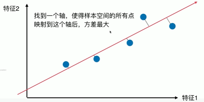
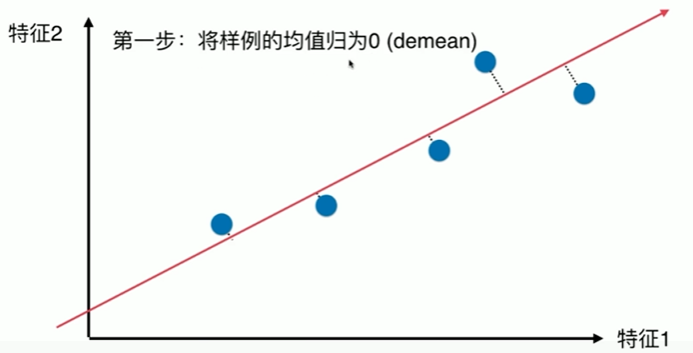
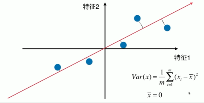
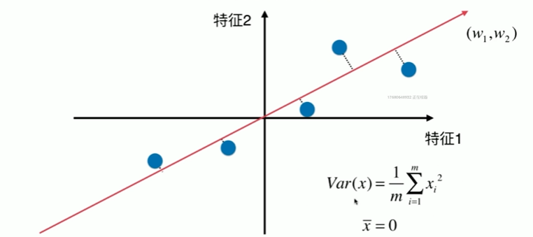
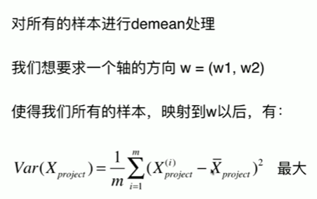

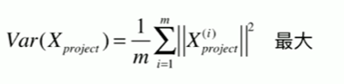
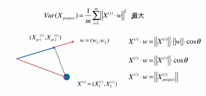
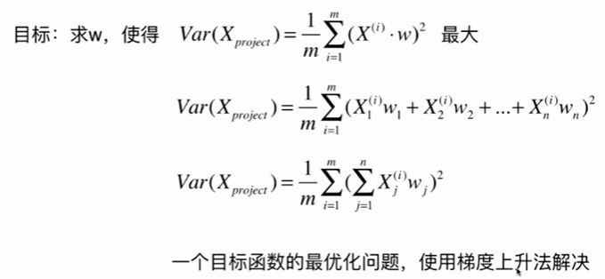
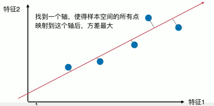
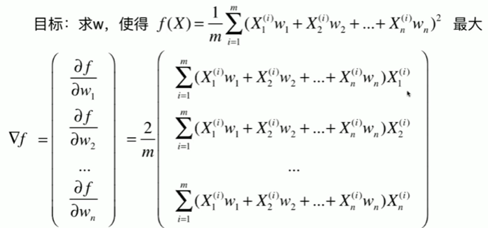
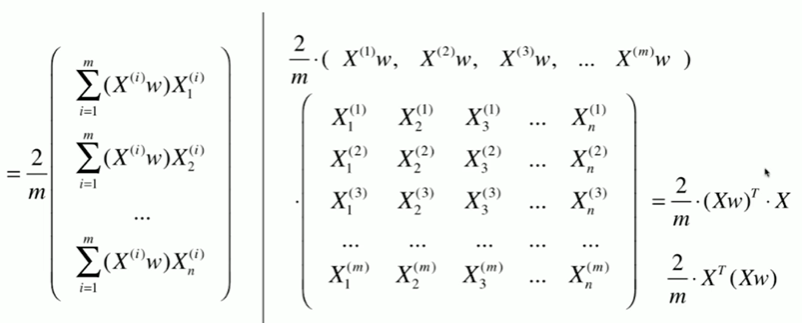
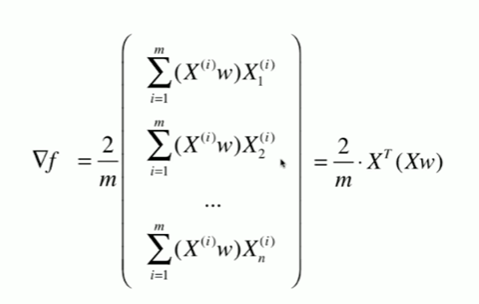
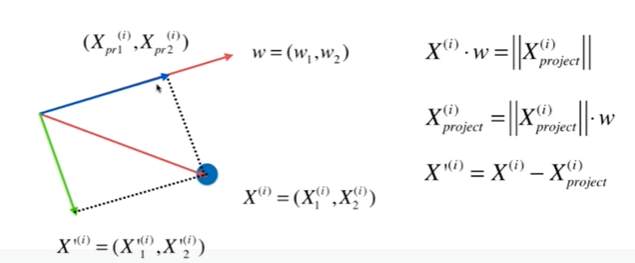
7-2 使用梯度上升法求解PCA问题
7-3 求数据的主成分PCA
Notbook 示例
Notbook 源码

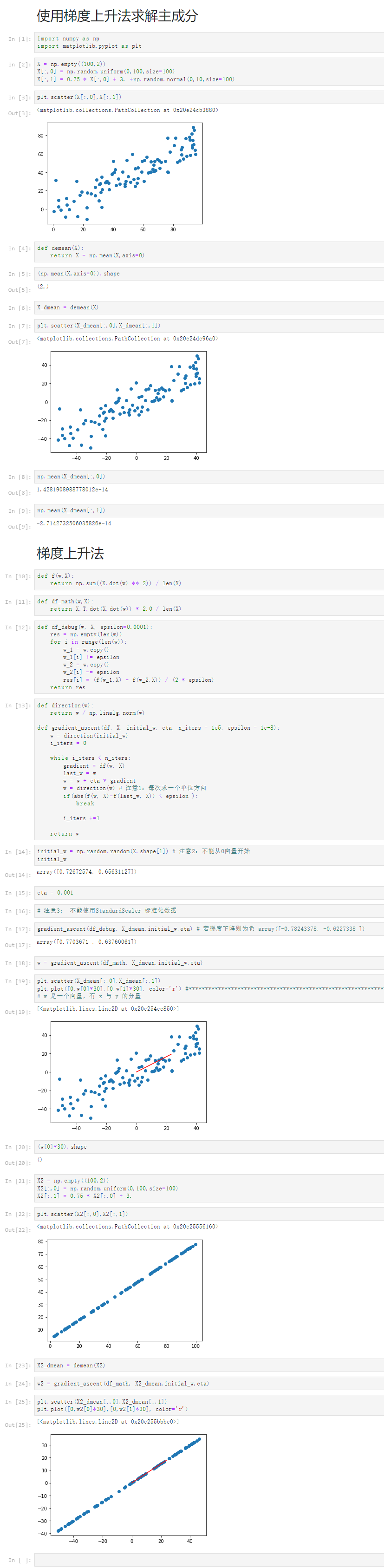
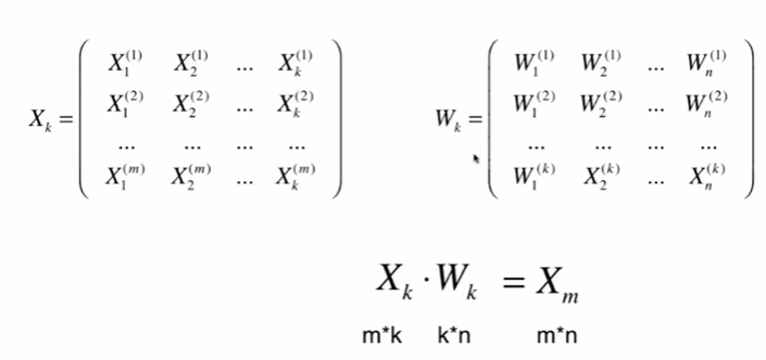
  1 使用梯度上升法求解主成分
  2 [1]
  3 import numpy as np
  4 import matplotlib.pyplot as plt
  5 [2]
  6 X = np.empty((100,2))
  7 X[:,0] = np.random.uniform(0,100,size=100)
  8 X[:,1] = 0.75 * X[:,0] + 3. +np.random.normal(0,10,size=100)
  9 [3]
 10 plt.scatter(X[:,0],X[:,1])
 11 <matplotlib.collections.PathCollection at 0x20e24cb3880>
 12
 13 [4]
 14 def demean(X):
 15     return X - np.mean(X,axis=0)
 16 [5]
 17 (np.mean(X,axis=0)).shape
 18 (2,)
 19 [6]
 20 X_dmean = demean(X)
 21 [7]
 22 plt.scatter(X_dmean[:,0],X_dmean[:,1])
 23 <matplotlib.collections.PathCollection at 0x20e24dc96a0>
 24
 25 [8]
 26 np.mean(X_dmean[:,0])
 27 1.4281908988778012e-14
 28 [9]
 29 np.mean(X_dmean[:,1])
 30 -2.7142732506035826e-14
 31 梯度上升法
 32 [10]
 33 def f(w,X):
 34     return np.sum((X.dot(w) ** 2)) / len(X)
 35 [11]
 36 def df_math(w,X):
 37     return X.T.dot(X.dot(w)) * 2.0 / len(X)
 38 [12]
 39 def df_debug(w, X, epsilon=0.0001):
 40     res = np.empty(len(w))
 41     for i in range(len(w)):
 42         w_1 = w.copy()
 43         w_1[i] += epsilon
 44         w_2 = w.copy()
 45         w_2[i] -= epsilon
 46         res[i] = (f(w_1,X) - f(w_2,X)) / (2 * epsilon)
 47     return res
 48 [13]
 49 def direction(w):
 50     return w / np.linalg.norm(w)
 51
 52 def gradient_ascent(df, X, initial_w, eta, n_iters = 1e5, epsilon = 1e-8):
 53     w = direction(initial_w)
 54     i_iters = 0
 55
 56     while i_iters < n_iters:
 57         gradient = df(w, X)
 58         last_w = w
 59         w = w + eta * gradient
 60         w = direction(w) # 注意1:每次求一个单位方向
 61         if(abs(f(w, X)-f(last_w, X)) < epsilon ):
 62             break
 63
 64         i_iters +=1
 65
 66     return w
 67 [14]
 68 initial_w = np.random.random(X.shape[1]) # 注意2:不能从0向量开始
 69 initial_w
 70 array([0.72672574, 0.65631127])
 71 [15]
 72 eta = 0.001
 73 [16]
 74 # 注意3: 不能使用StandardScaler 标准化数据
 75 [17]
 76 gradient_ascent(df_debug, X_dmean,initial_w,eta) # 若梯度下降则为负 array([-0.78243378, -0.6227338 ])
 77 array([0.7703671 , 0.63760061])
 78 [18]
 79 w = gradient_ascent(df_math, X_dmean,initial_w,eta)
 80 [19]
 81 plt.scatter(X_dmean[:,0],X_dmean[:,1])
 82 plt.plot([0,w[0]*30],[0,w[1]*30], color='r') #***********************************************************************
 83 # w 是一个向量,有 x 与 y 的分量
 84 [<matplotlib.lines.Line2D at 0x20e254ec850>]
 85
 86 [20]
 87 (w[0]*30).shape
 88 ()
 89 [21]
 90 X2 = np.empty((100,2))
 91 X2[:,0] = np.random.uniform(0,100,size=100)
 92 X2[:,1] = 0.75 * X2[:,0] + 3.
 93 [22]
 94 plt.scatter(X2[:,0],X2[:,1])
 95 <matplotlib.collections.PathCollection at 0x20e25556160>
 96
 97 [23]
 98 X2_dmean = demean(X2)
 99 [24]
100 w2 = gradient_ascent(df_math, X2_dmean,initial_w,eta)
101 [25]
102 plt.scatter(X2_dmean[:,0],X2_dmean[:,1])
103 plt.plot([0,w2[0]*30],[0,w2[1]*30], color='r')
104 [<matplotlib.lines.Line2D at 0x20e255bbbe0>]
7-4 求数据的前n个主成分

Notbook 示例
Notbook 源码
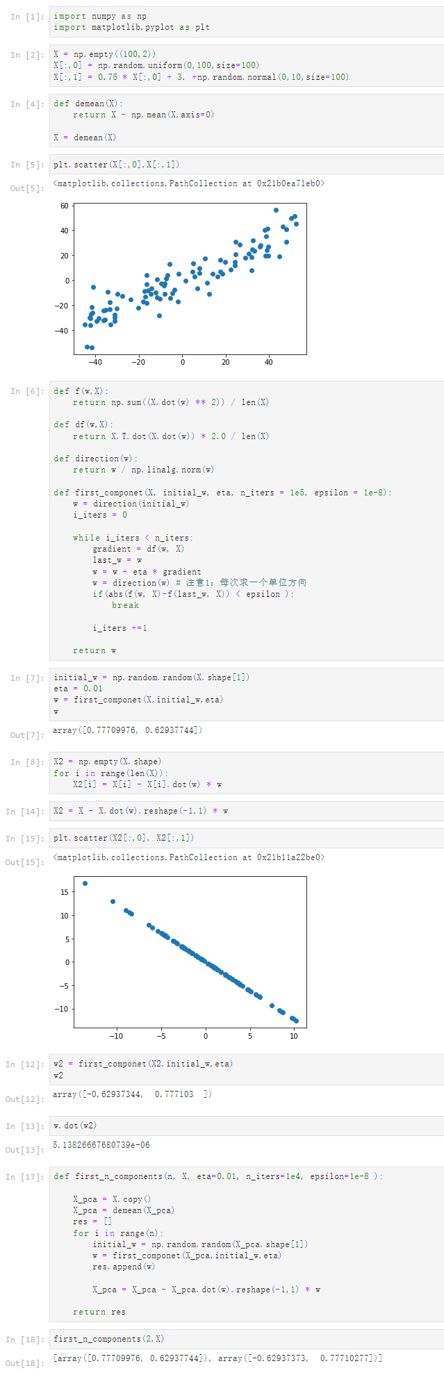
 1 [1]
 2 import numpy as np
 3 import matplotlib.pyplot as plt
 4 [2]
 5 X = np.empty((100,2))
 6 X[:,0] = np.random.uniform(0,100,size=100)
 7 X[:,1] = 0.75 * X[:,0] + 3. +np.random.normal(0,10,size=100)
 8 [4]
 9 def demean(X):
10     return X - np.mean(X,axis=0)
11
12 X = demean(X)
13 [5]
14 plt.scatter(X[:,0],X[:,1])
15 <matplotlib.collections.PathCollection at 0x21b0ea71eb0>
16
17 [6]
18 def f(w,X):
19     return np.sum((X.dot(w) ** 2)) / len(X)
20
21 def df(w,X):
22     return X.T.dot(X.dot(w)) * 2.0 / len(X)
23
24 def direction(w):
25     return w / np.linalg.norm(w)
26
27 def first_componet(X, initial_w, eta, n_iters = 1e5, epsilon = 1e-8):
28     w = direction(initial_w)
29     i_iters = 0
30
31     while i_iters < n_iters:
32         gradient = df(w, X)
33         last_w = w
34         w = w + eta * gradient
35         w = direction(w) # 注意1:每次求一个单位方向
36         if(abs(f(w, X)-f(last_w, X)) < epsilon ):
37             break
38
39         i_iters +=1
40
41     return w
42 [7]
43 initial_w = np.random.random(X.shape[1])
44 eta = 0.01
45 w = first_componet(X,initial_w,eta)
46 w
47 array([0.77709976, 0.62937744])
48 [8]
49 X2 = np.empty(X.shape)
50 for i in range(len(X)):
51     X2[i] = X[i] - X[i].dot(w) * w
52 [14]
53 X2 = X - X.dot(w).reshape(-1,1) * w
54 [15]
55 plt.scatter(X2[:,0], X2[:,1])
56 <matplotlib.collections.PathCollection at 0x21b11a22be0>
57
58 [12]
59 w2 = first_componet(X2,initial_w,eta)
60 w2
61 array([-0.62937344,  0.777103  ])
62 [13]
63 w.dot(w2)
64 5.13826667680739e-06
65 [17]
66 def first_n_components(n, X, eta=0.01, n_iters=1e4, epsilon=1e-8 ):
67
68     X_pca = X.copy()
69     X_pca = demean(X_pca)
70     res = []
71     for i in range(n):
72         initial_w = np.random.random(X_pca.shape[1])
73         w = first_componet(X_pca,initial_w,eta)
74         res.append(w)
75
76         X_pca = X_pca - X_pca.dot(w).reshape(-1,1) * w
77
78     return res
79 [18]
80 first_n_components(2,X)
81 [array([0.77709976, 0.62937744]), array([-0.62937373,  0.77710277])]
7-5 高维数据映射为低维数据
Notbook 示例
Notbook 源码
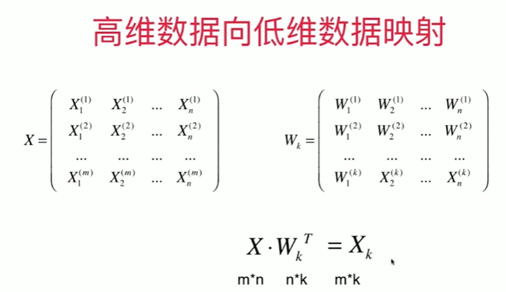
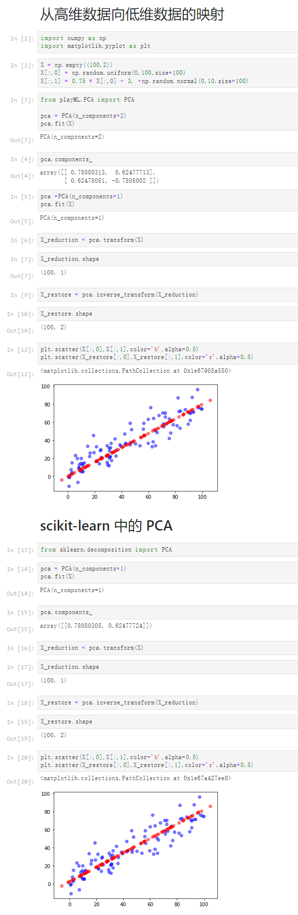
 1 从高维数据向低维数据的映射
 2 [1]
 3 import numpy as np
 4 import matplotlib.pyplot as plt
 5 [2]
 6 X = np.empty((100,2))
 7 X[:,0] = np.random.uniform(0,100,size=100)
 8 X[:,1] = 0.75 * X[:,0] + 3. +np.random.normal(0,10,size=100)
 9 [3]
10 from playML.PCA import PCA
11
12 pca = PCA(n_components=2)
13 pca.fit(X)
14 PCA(n_components=2)
15 [4]
16 pca.components_
17 array([[ 0.78080313,  0.62477713],
18        [ 0.62478081, -0.7808002 ]])
19 [5]
20 pca =PCA(n_components=1)
21 pca.fit(X)
22 PCA(n_components=1)
23 [6]
24 X_reduction = pca.transform(X)
25 [7]
26 X_reduction.shape
27 (100, 1)
28 [9]
29 X_restore = pca.inverse_transform(X_reduction)
30 [10]
31 X_restore.shape
32 (100, 2)
33 [12]
34 plt.scatter(X[:,0],X[:,1],color='b',alpha=0.5)
35 plt.scatter(X_restore[:,0],X_restore[:,1],color='r',alpha=0.5)
36 <matplotlib.collections.PathCollection at 0x1e67905a550>
37
38 scikit-learn 中的 PCA
39 [13]
40 from sklearn.decomposition import PCA
41 [14]
42 pca = PCA(n_components=1)
43 pca.fit(X)
44 PCA(n_components=1)
45 [15]
46 pca.components_
47 array([[0.78080305, 0.62477724]])
48 [16]
49 X_reduction = pca.transform(X)
50 [17]
51 X_reduction.shape
52 (100, 1)
53 [18]
54 X_restore = pca.inverse_transform(X_reduction)
55 [19]
56 X_restore.shape
57 (100, 2)
58 [20]
59 plt.scatter(X[:,0],X[:,1],color='b',alpha=0.5)
60 plt.scatter(X_restore[:,0],X_restore[:,1],color='r',alpha=0.5)
61 <matplotlib.collections.PathCollection at 0x1e67a427ee0>
7-6 scikit-learn中的PCA
Notbook 示例
notbook 源码
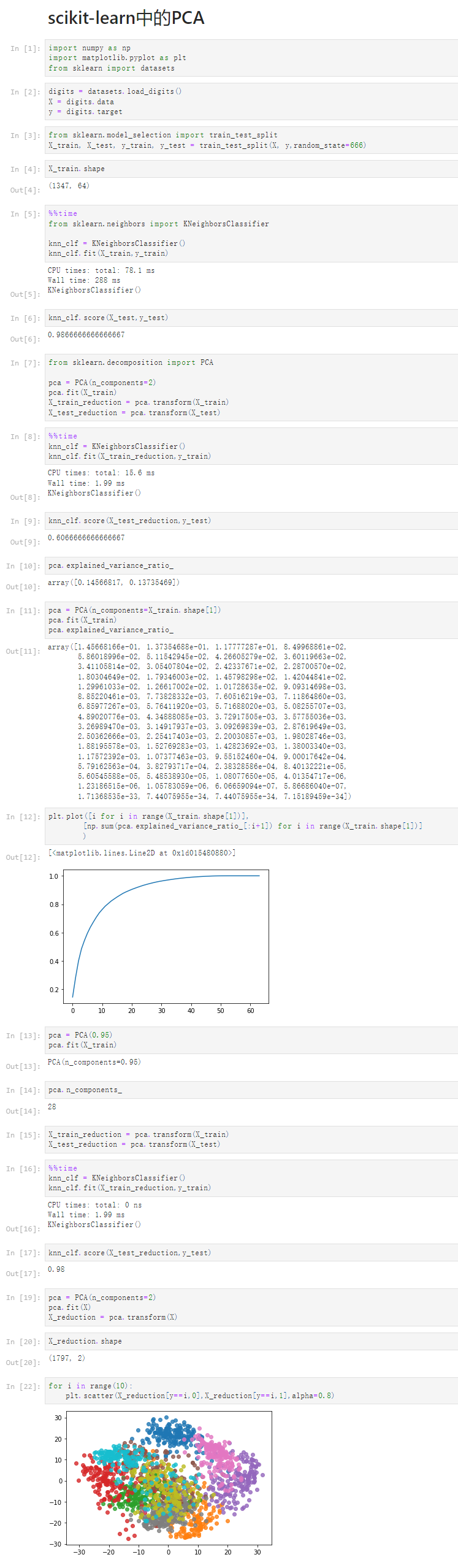
  1 scikit-learn中的PCA
  2 [1]
  3 import numpy as np
  4 import matplotlib.pyplot as plt
  5 from sklearn import datasets
  6 [2]
  7 digits = datasets.load_digits()
  8 X = digits.data
  9 y = digits.target
 10 [3]
 11 from sklearn.model_selection import train_test_split
 12 X_train, X_test, y_train, y_test = train_test_split(X, y,random_state=666)
 13 [4]
 14 X_train.shape
 15 (1347, 64)
 16 [5]
 17 %%time
 18 from sklearn.neighbors import KNeighborsClassifier
 19
 20 knn_clf = KNeighborsClassifier()
 21 knn_clf.fit(X_train,y_train)
 22 CPU times: total: 78.1 ms
 23 Wall time: 288 ms
 24
 25 KNeighborsClassifier()
 26 [6]
 27 knn_clf.score(X_test,y_test)
 28 0.9866666666666667
 29 [7]
 30 from sklearn.decomposition import PCA
 31
 32 pca = PCA(n_components=2)
 33 pca.fit(X_train)
 34 X_train_reduction = pca.transform(X_train)
 35 X_test_reduction = pca.transform(X_test)
 36 [8]
 37 %%time
 38 knn_clf = KNeighborsClassifier()
 39 knn_clf.fit(X_train_reduction,y_train)
 40 CPU times: total: 15.6 ms
 41 Wall time: 1.99 ms
 42
 43 KNeighborsClassifier()
 44 [9]
 45 knn_clf.score(X_test_reduction,y_test)
 46 0.6066666666666667
 47 [10]
 48 pca.explained_variance_ratio_
 49 array([0.14566817, 0.13735469])
 50 [11]
 51 pca = PCA(n_components=X_train.shape[1])
 52 pca.fit(X_train)
 53 pca.explained_variance_ratio_
 54 array([1.45668166e-01, 1.37354688e-01, 1.17777287e-01, 8.49968861e-02,
 55        5.86018996e-02, 5.11542945e-02, 4.26605279e-02, 3.60119663e-02,
 56        3.41105814e-02, 3.05407804e-02, 2.42337671e-02, 2.28700570e-02,
 57        1.80304649e-02, 1.79346003e-02, 1.45798298e-02, 1.42044841e-02,
 58        1.29961033e-02, 1.26617002e-02, 1.01728635e-02, 9.09314698e-03,
 59        8.85220461e-03, 7.73828332e-03, 7.60516219e-03, 7.11864860e-03,
 60        6.85977267e-03, 5.76411920e-03, 5.71688020e-03, 5.08255707e-03,
 61        4.89020776e-03, 4.34888085e-03, 3.72917505e-03, 3.57755036e-03,
 62        3.26989470e-03, 3.14917937e-03, 3.09269839e-03, 2.87619649e-03,
 63        2.50362666e-03, 2.25417403e-03, 2.20030857e-03, 1.98028746e-03,
 64        1.88195578e-03, 1.52769283e-03, 1.42823692e-03, 1.38003340e-03,
 65        1.17572392e-03, 1.07377463e-03, 9.55152460e-04, 9.00017642e-04,
 66        5.79162563e-04, 3.82793717e-04, 2.38328586e-04, 8.40132221e-05,
 67        5.60545588e-05, 5.48538930e-05, 1.08077650e-05, 4.01354717e-06,
 68        1.23186515e-06, 1.05783059e-06, 6.06659094e-07, 5.86686040e-07,
 69        1.71368535e-33, 7.44075955e-34, 7.44075955e-34, 7.15189459e-34])
 70 [12]
 71 plt.plot([i for i in range(X_train.shape[1])],
 72         [np.sum(pca.explained_variance_ratio_[:i+1]) for i in range(X_train.shape[1])]
 73         )
 74 [<matplotlib.lines.Line2D at 0x1d015480880>]
 75
 76 [13]
 77 pca = PCA(0.95)
 78 pca.fit(X_train)
 79 PCA(n_components=0.95)
 80 [14]
 81 pca.n_components_
 82 28
 83 [15]
 84 X_train_reduction = pca.transform(X_train)
 85 X_test_reduction = pca.transform(X_test)
 86 [16]
 87 %%time
 88 knn_clf = KNeighborsClassifier()
 89 knn_clf.fit(X_train_reduction,y_train)
 90 CPU times: total: 0 ns
 91 Wall time: 1.99 ms
 92
 93 KNeighborsClassifier()
 94 [17]
 95 knn_clf.score(X_test_reduction,y_test)
 96 0.98
 97 [19]
 98 pca = PCA(n_components=2)
 99 pca.fit(X)
100 X_reduction = pca.transform(X)
101 [20]
102 X_reduction.shape
103 (1797, 2)
104 [22]
105 for i in range(10):
106     plt.scatter(X_reduction[y==i,0],X_reduction[y==i,1],alpha=0.8)
7-7 试手MNIST数据集
Notbook 示例
Notbook 源码
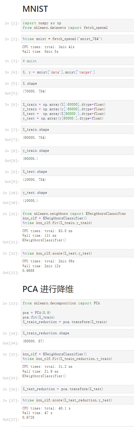
 1 MNIST
 2 [1]
 3 import numpy as np
 4 from sklearn.datasets import fetch_openml
 5 [2]
 6 %time mnist = fetch_openml('mnist_784')
 7 CPU times: total: 3min 41s
 8 Wall time: 5min 5s
 9
10 [3]
11 # mnist
12 [4]
13 X, y = mnist['data'],mnist['target']
14 [5]
15 X.shape
16 (70000, 784)
17 [6]
18 X_train = np.array(X[:60000],dtype=float)
19 y_train = np.array(y[:60000],dtype=float)
20 X_test =  np.array(X[60000:],dtype=float)
21 y_test = np.array(y[60000:],dtype=float)
22 [7]
23 X_train.shape
24 (60000, 784)
25 [8]
26 y_train.shape
27 (60000,)
28 [9]
29 X_test.shape
30 (10000, 784)
31 [10]
32 y_test.shape
33 (10000,)
34 [11]
35 from sklearn.neighbors import KNeighborsClassifier
36 knn_clf = KNeighborsClassifier()
37 %time knn_clf.fit(X_train,y_train)
38 CPU times: total: 93.8 ms
39 Wall time: 131 ms
40
41 KNeighborsClassifier()
42 [12]
43 %time knn_clf.score(X_test,y_test)
44 CPU times: total: 2min 56s
45 Wall time: 2min 12s
46
47 0.9688
48 PCA 进行降维
49 [13]
50 from sklearn.decomposition import PCA
51
52 pca = PCA(0.9)
53 pca.fit(X_train)
54 X_train_reduction = pca.transform(X_train)
55 [14]
56 X_train_reduction.shape
57 (60000, 87)
58 [15]
59 knn_clf = KNeighborsClassifier()
60 %time knn_clf.fit(X_train_reduction,y_train)
61 CPU times: total: 31.2 ms
62 Wall time: 21.9 ms
63
64 KNeighborsClassifier()
65 [16]
66 X_test_reduction = pca.transform(X_test)
67 [17]
68 %time knn_clf.score(X_test_reduction,y_test)
69 CPU times: total: 40.1 s
70 Wall time: 47 s
71
72 0.9728
7-8 使用PCA对数据进行降噪
Notbook 示例
Notbook 源码
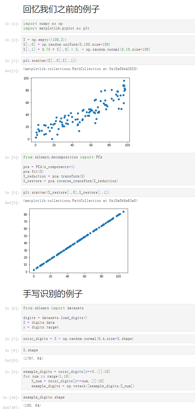
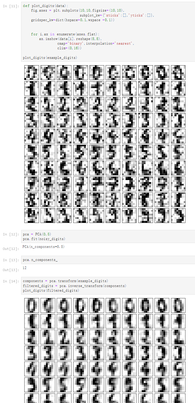
回忆我们之前的例子
[1]
import numpy as np
import matplotlib.pyplot as plt
[2]
X = np.empty((100,2))
X[:,0] = np.random.uniform(0,100,size=100)
X[:,1] = 0.75 * X[:,0] + 3. + np.random.normal(0,10,size=100)
[3]
plt.scatter(X[:,0],X[:,1])
<matplotlib.collections.PathCollection at 0x18a08e43820>

[4]
from sklearn.decomposition import PCA

pca = PCA(n_components=1)
pca.fit(X)
X_reduction = pca.transform(X)
X_restore = pca.inverse_transform(X_reduction)
[5]
plt.scatter(X_restore[:,0],X_restore[:,1])
<matplotlib.collections.PathCollection at 0x18a0b8a63a0>

手写识别的例子
[6]
from sklearn import datasets

digits = datasets.load_digits()
X = digits.data
y = digits.target
[7]
noisy_digits = X + np.random.normal(0,4,size=X.shape)
[8]
X.shape
(1797, 64)
[9]
example_digits = noisy_digits[y==0,:][:10]
for num in range(1,10):
    X_num = noisy_digits[y==num,:][:10]
    example_digits = np.vstack([example_digits,X_num])
[10]
example_digits.shape
(100, 64)
[11]
def plot_digits(data):
    fig,axes = plt.subplots(10,10,figsize=(10,10),
                            subplot_kw={'xticks':[],'yticks':[]},
    gridspec_kw=dict(hspace=0.1,wspace =0.1))


    for i,ax in enumerate(axes.flat):
        ax.imshow(data[i].reshape(8,8),
                 cmap='binary',interpolation='nearest',
                 clim=(0,16))

plot_digits(example_digits)

[12]
pca = PCA(0.5)
pca.fit(noisy_digits)
PCA(n_components=0.5)
[13]
pca.n_components_
12
[14]
components = pca.transform(example_digits)
filtered_digits = pca.inverse_transform(components)
plot_digits(filtered_digits)
7-9 人脸识别与特征脸
Notbook 示例
Notbook 源码
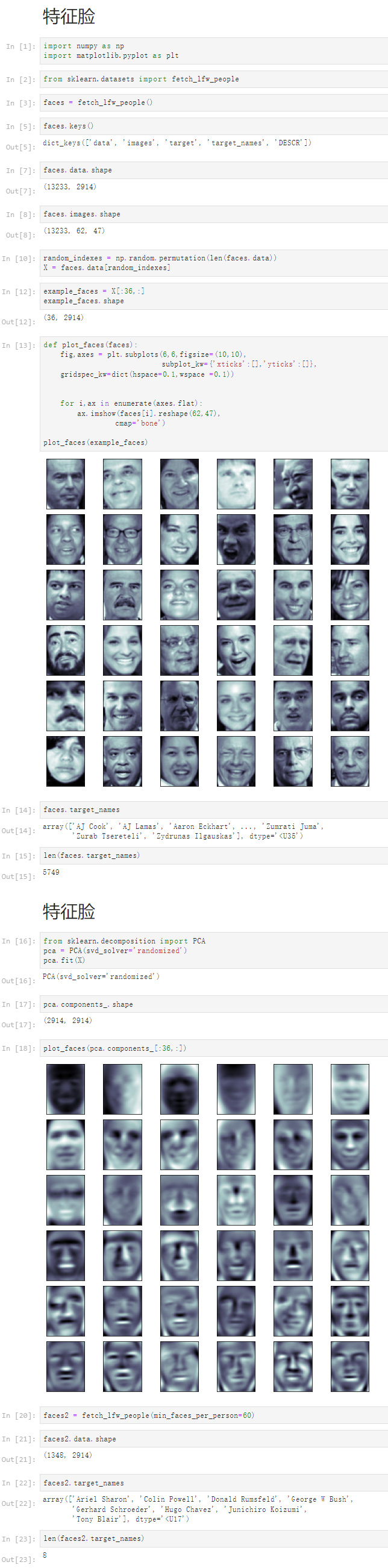
 1 特征脸
 2 [1]
 3 import numpy as np
 4 import matplotlib.pyplot as plt
 5 [2]
 6 from sklearn.datasets import fetch_lfw_people
 7 [3]
 8 faces = fetch_lfw_people()
 9 [5]
10 faces.keys()
11 dict_keys(['data', 'images', 'target', 'target_names', 'DESCR'])
12 [7]
13 faces.data.shape
14 (13233, 2914)
15 [8]
16 faces.images.shape
17 (13233, 62, 47)
18 [10]
19 random_indexes = np.random.permutation(len(faces.data))
20 X = faces.data[random_indexes]
21 [12]
22 example_faces = X[:36,:]
23 example_faces.shape
24 (36, 2914)
25 [13]
26 def plot_faces(faces):
27     fig,axes = plt.subplots(6,6,figsize=(10,10),
28                             subplot_kw={'xticks':[],'yticks':[]},
29     gridspec_kw=dict(hspace=0.1,wspace =0.1))
30
31
32     for i,ax in enumerate(axes.flat):
33         ax.imshow(faces[i].reshape(62,47),
34                  cmap='bone')
35
36 plot_faces(example_faces)
37
38 [14]
39 faces.target_names
40 array(['AJ Cook', 'AJ Lamas', 'Aaron Eckhart', ..., 'Zumrati Juma',
41        'Zurab Tsereteli', 'Zydrunas Ilgauskas'], dtype='<U35')
42 [15]
43 len(faces.target_names)
44 5749
45 特征脸
46 [16]
47 from sklearn.decomposition import PCA
48 pca = PCA(svd_solver='randomized')
49 pca.fit(X)
50 PCA(svd_solver='randomized')
51 [17]
52 pca.components_.shape
53 (2914, 2914)
54 [18]
55 plot_faces(pca.components_[:36,:])
56
57 [20]
58 faces2 = fetch_lfw_people(min_faces_per_person=60)
59 [21]
60 faces2.data.shape
61 (1348, 2914)
62 [22]
63 faces2.target_names
64 array(['Ariel Sharon', 'Colin Powell', 'Donald Rumsfeld', 'George W Bush',
65        'Gerhard Schroeder', 'Hugo Chavez', 'Junichiro Koizumi',
66        'Tony Blair'], dtype='<U17')
67 [23]
68 len(faces2.target_names)
69 8


【推荐】国内首个AI IDE,深度理解中文开发场景,立即下载体验Trae
【推荐】编程新体验,更懂你的AI,立即体验豆包MarsCode编程助手
【推荐】抖音旗下AI助手豆包,你的智能百科全书,全免费不限次数
【推荐】轻量又高性能的 SSH 工具 IShell:AI 加持,快人一步
· TypeScript + Deepseek 打造卜卦网站:技术与玄学的结合
· 阿里巴巴 QwQ-32B真的超越了 DeepSeek R-1吗?
· 【译】Visual Studio 中新的强大生产力特性
· 【设计模式】告别冗长if-else语句:使用策略模式优化代码结构
· 10年+ .NET Coder 心语 ── 封装的思维:从隐藏、稳定开始理解其本质意义