第5章上 线性回归法

 

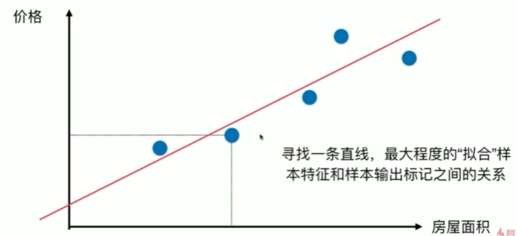
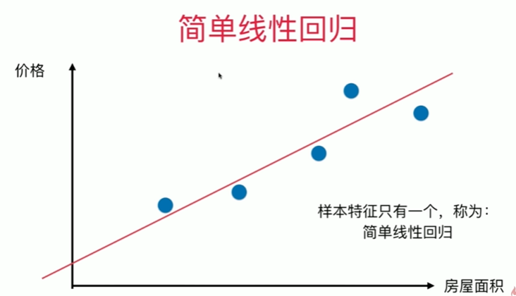
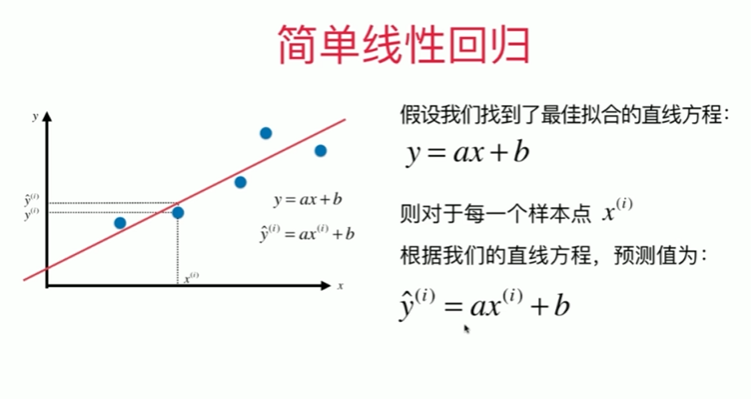
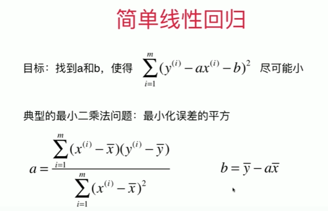
5-1 简单线性回归

 

 

 

 

 

 

 

 

 

 

 

 

 

 

 

 

 

 

 

 

 

 

 

 

 

 

 

 

 

 

 

 

 

 

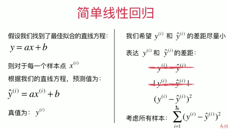
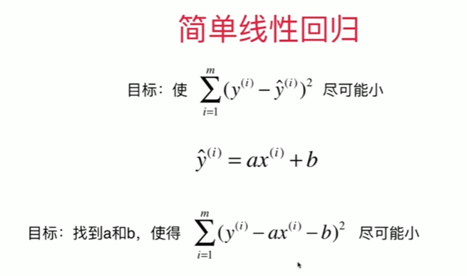
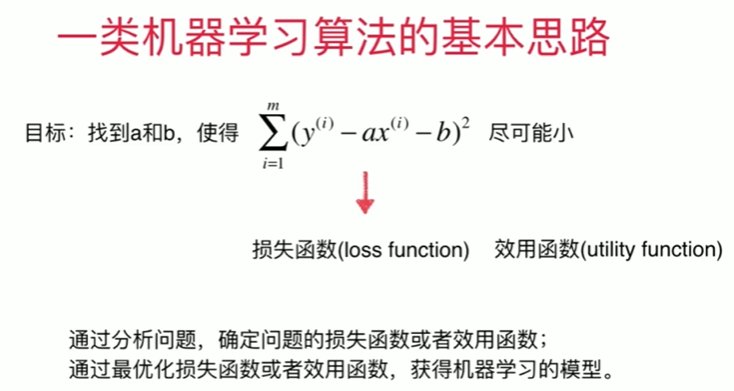
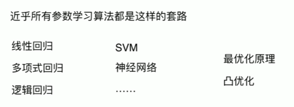
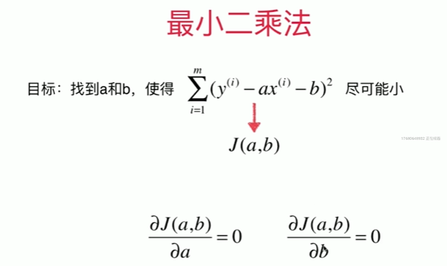
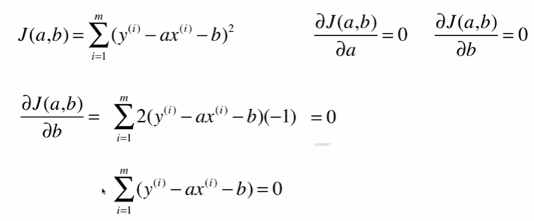
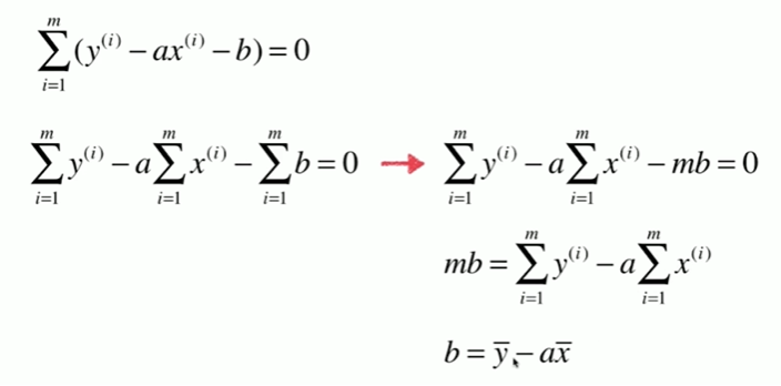
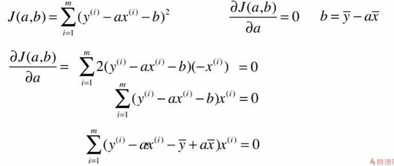
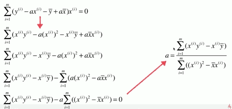
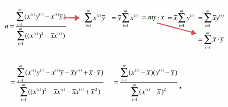
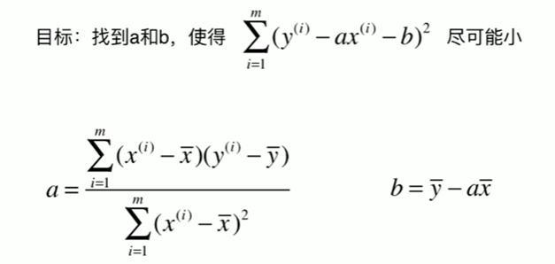
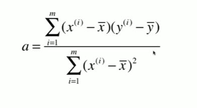
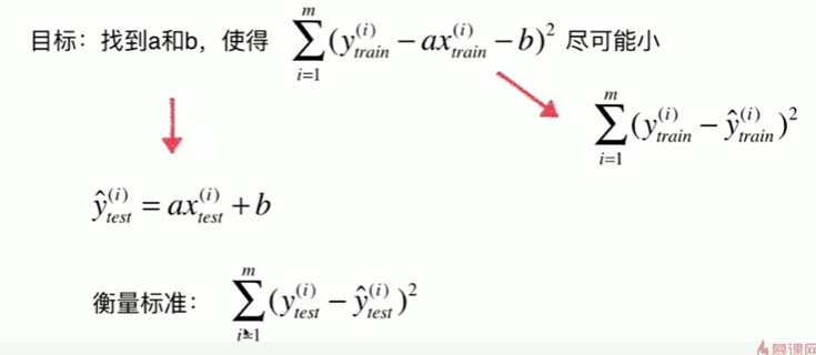
 5-2 最小二乘法

 

 

 

 

 

 

 

 

 

 

 

 

 

 

 

 

 

 

 

 

 

 

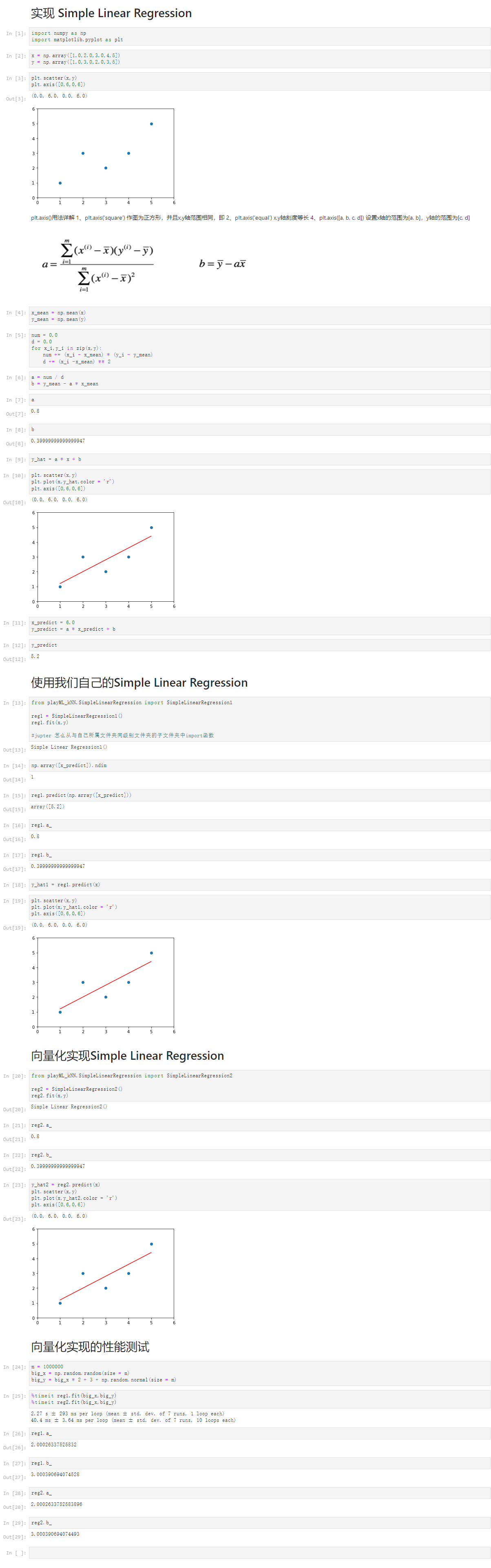
5-3 简单线性回归的实现

#见下面代码

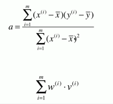
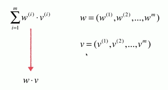
5-4 向量化

 

 

 

 

 

 

 

 

 

 

 

 

Notbook 示例

Notbook 源码

实现 Simple Linear Regression
[1]
import numpy as np
import matplotlib.pyplot as plt
[2]
x = np.array([1.0,2.0,3.0,4,5])
y = np.array([1.0,3.0,2.0,3,5])
[3]
plt.scatter(x,y)
plt.axis([0,6,0,6])
(0.0, 6.0, 0.0, 6.0)

plt.axis()用法详解 1、plt.axis(‘square’) 作图为正方形，并且x,y轴范围相同，即 2、plt.axis(‘equal’) x,y轴刻度等长 4、plt.axis([a, b, c, d]) 设置x轴的范围为[a, b]，y轴的范围为[c, d]

%E7%BA%BF%E6%80%A7%E5%9B%9E%E5%BD%92.png

[4]
x_mean = np.mean(x)
y_mean = np.mean(y)
[5]
num = 0.0
d = 0.0
for x_i,y_i in zip(x,y):
    num += (x_i - x_mean) * (y_i - y_mean)
    d += (x_i -x_mean) ** 2
[6]
a = num / d
b = y_mean - a * x_mean
[7]
a
0.8
[8]
b
0.39999999999999947
[9]
y_hat = a * x + b
[10]
plt.scatter(x,y)
plt.plot(x,y_hat,color = 'r')
plt.axis([0,6,0,6])
(0.0, 6.0, 0.0, 6.0)

[11]
x_predict = 6.0
y_predict = a * x_predict + b
[12]
y_predict
5.2
使用我们自己的Simple Linear Regression
[13]
from playML_kNN.SimpleLinearRegression import SimpleLinearRegression1

reg1 = SimpleLinearRegression1()
reg1.fit(x,y)

#jupter 怎么从与自己所属文件夹同级别文件夹的子文件夹中import函数
Simple Linear Regression1()
[14]
np.array([x_predict]).ndim
1
[15]
reg1.predict(np.array([x_predict]))
array([5.2])
[16]
reg1.a_
0.8
[17]
reg1.b_
0.39999999999999947
[18]
y_hat1 = reg1.predict(x)
[19]
plt.scatter(x,y)
plt.plot(x,y_hat1,color = 'r')
plt.axis([0,6,0,6])
(0.0, 6.0, 0.0, 6.0)

向量化实现Simple Linear Regression
[20]
from playML_kNN.SimpleLinearRegression import SimpleLinearRegression2

reg2 = SimpleLinearRegression2()
reg2.fit(x,y)
Simple Linear Regression2()
[21]
reg2.a_
0.8
[22]
reg2.b_
0.39999999999999947
[23]
y_hat2 = reg2.predict(x)
plt.scatter(x,y)
plt.plot(x,y_hat2,color = 'r')
plt.axis([0,6,0,6])
(0.0, 6.0, 0.0, 6.0)

向量化实现的性能测试
[24]
m = 1000000
big_x = np.random.random(size = m)
big_y = big_x * 2 + 3 + np.random.normal(size = m)
[25]
%timeit reg1.fit(big_x,big_y)
%timeit reg2.fit(big_x,big_y)
2.27 s ± 293 ms per loop (mean ± std. dev. of 7 runs, 1 loop each)
40.4 ms ± 3.64 ms per loop (mean ± std. dev. of 7 runs, 10 loops each)

[26]
reg1.a_
2.00026337525832
[27]
reg1.b_
3.000390694074528
[28]
reg2.a_
2.0002633752583896
[29]
reg2.b_
3.000390694074493

 

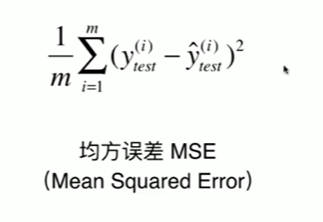
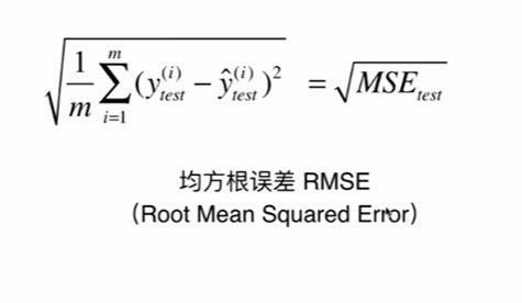
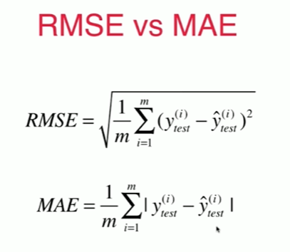
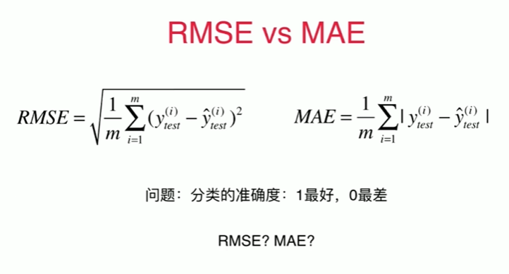
5-5 衡量线性回归法的指标 MSE,RMS,MAE

 

 

 

 

 

 

 

 

 

 

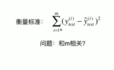
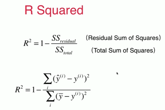
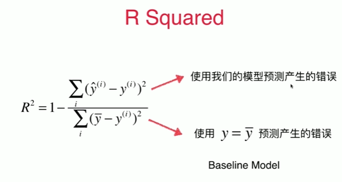
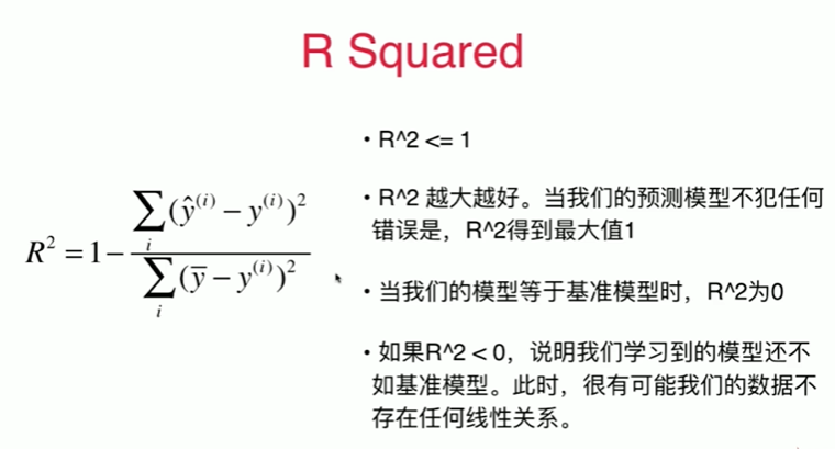
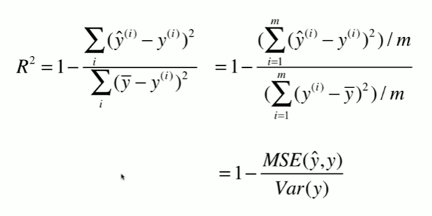
 5-6 最好的衡量线性回归法的指标 R Squared

 

 

 

 

 

 

 

 

 

Notbook 示例

 

 

Notbook 源码

 

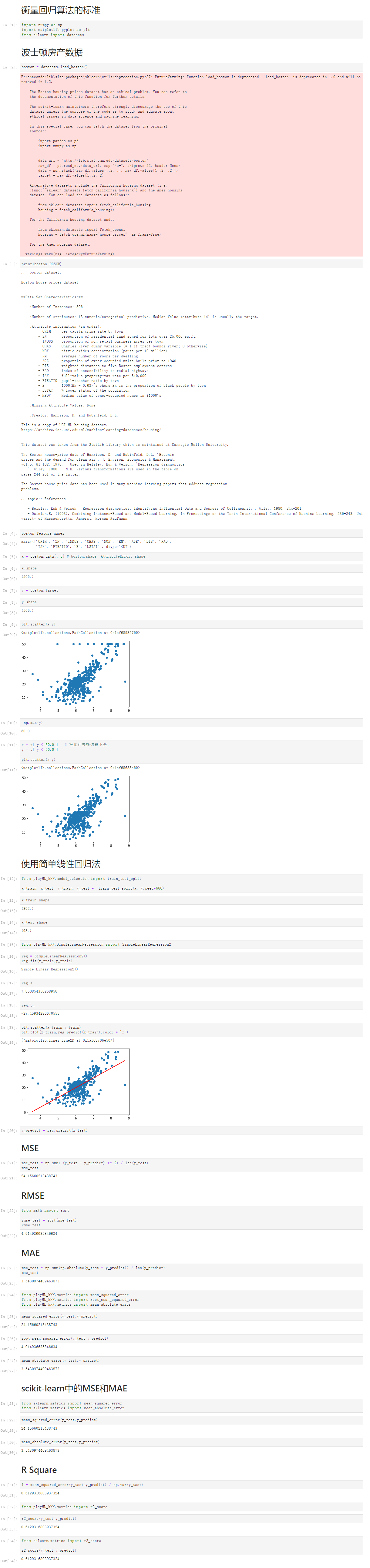
衡量回归算法的标准
[1]
import numpy as np
import matplotlib.pyplot as plt
from sklearn import datasets
波士顿房产数据
[2]
boston = datasets.load_boston()
F:\anaconda\lib\site-packages\sklearn\utils\deprecation.py:87: FutureWarning: Function load_boston is deprecated; `load_boston` is deprecated in 1.0 and will be removed in 1.2.

    The Boston housing prices dataset has an ethical problem. You can refer to
    the documentation of this function for further details.

    The scikit-learn maintainers therefore strongly discourage the use of this
    dataset unless the purpose of the code is to study and educate about
    ethical issues in data science and machine learning.

    In this special case, you can fetch the dataset from the original
    source::

        import pandas as pd
        import numpy as np


        data_url = "http://lib.stat.cmu.edu/datasets/boston"
        raw_df = pd.read_csv(data_url, sep="\s+", skiprows=22, header=None)
        data = np.hstack([raw_df.values[::2, :], raw_df.values[1::2, :2]])
        target = raw_df.values[1::2, 2]

    Alternative datasets include the California housing dataset (i.e.
    :func:`~sklearn.datasets.fetch_california_housing`) and the Ames housing
    dataset. You can load the datasets as follows::

        from sklearn.datasets import fetch_california_housing
        housing = fetch_california_housing()

    for the California housing dataset and::

        from sklearn.datasets import fetch_openml
        housing = fetch_openml(name="house_prices", as_frame=True)

    for the Ames housing dataset.
    
  warnings.warn(msg, category=FutureWarning)

[3]
print(boston.DESCR)
.. _boston_dataset:

Boston house prices dataset
---------------------------

**Data Set Characteristics:**  

    :Number of Instances: 506 

    :Number of Attributes: 13 numeric/categorical predictive. Median Value (attribute 14) is usually the target.

    :Attribute Information (in order):
        - CRIM     per capita crime rate by town
        - ZN       proportion of residential land zoned for lots over 25,000 sq.ft.
        - INDUS    proportion of non-retail business acres per town
        - CHAS     Charles River dummy variable (= 1 if tract bounds river; 0 otherwise)
        - NOX      nitric oxides concentration (parts per 10 million)
        - RM       average number of rooms per dwelling
        - AGE      proportion of owner-occupied units built prior to 1940
        - DIS      weighted distances to five Boston employment centres
        - RAD      index of accessibility to radial highways
        - TAX      full-value property-tax rate per $10,000
        - PTRATIO  pupil-teacher ratio by town
        - B        1000(Bk - 0.63)^2 where Bk is the proportion of black people by town
        - LSTAT    % lower status of the population
        - MEDV     Median value of owner-occupied homes in $1000's

    :Missing Attribute Values: None

    :Creator: Harrison, D. and Rubinfeld, D.L.

This is a copy of UCI ML housing dataset.
https://archive.ics.uci.edu/ml/machine-learning-databases/housing/


This dataset was taken from the StatLib library which is maintained at Carnegie Mellon University.

The Boston house-price data of Harrison, D. and Rubinfeld, D.L. 'Hedonic
prices and the demand for clean air', J. Environ. Economics & Management,
vol.5, 81-102, 1978.   Used in Belsley, Kuh & Welsch, 'Regression diagnostics
...', Wiley, 1980.   N.B. Various transformations are used in the table on
pages 244-261 of the latter.

The Boston house-price data has been used in many machine learning papers that address regression
problems.   
     
.. topic:: References

   - Belsley, Kuh & Welsch, 'Regression diagnostics: Identifying Influential Data and Sources of Collinearity', Wiley, 1980. 244-261.
   - Quinlan,R. (1993). Combining Instance-Based and Model-Based Learning. In Proceedings on the Tenth International Conference of Machine Learning, 236-243, University of Massachusetts, Amherst. Morgan Kaufmann.


[4]
boston.feature_names
array(['CRIM', 'ZN', 'INDUS', 'CHAS', 'NOX', 'RM', 'AGE', 'DIS', 'RAD',
       'TAX', 'PTRATIO', 'B', 'LSTAT'], dtype='<U7')
[5]
x = boston.data[:,5] # boston.shape  AttributeError: shape
[6]
x.shape
(506,)
[7]
y = boston.target
[8]
y.shape
(506,)
[9]
plt.scatter(x,y)
<matplotlib.collections.PathCollection at 0x1af68582760>

[10]
 np.max(y)
50.0
[11]
x = x[ y < 50.0 ]   # 将此行去掉结果不变，
y = y[ y < 50.0 ]

plt.scatter(x,y)
<matplotlib.collections.PathCollection at 0x1af68688a60>

使用简单线性回归法
[12]
from playML_kNN.model_selection import train_test_split

x_train, x_test, y_train, y_test =  train_test_split(x, y,seed=666)
[13]
x_train.shape
(392,)
[14]
x_test.shape
(98,)
[15]
from playML_kNN.SimpleLinearRegression import SimpleLinearRegression2
[16]
reg = SimpleLinearRegression2()
reg.fit(x_train,y_train)
Simple Linear Regression2()
[17]
reg.a_
7.860854356268956
[18]
reg.b_
-27.45934280670555
[19]
plt.scatter(x_train,y_train)
plt.plot(x_train,reg.predict(x_train),color = 'r')
[<matplotlib.lines.Line2D at 0x1af68706e50>]

[20]
y_predict = reg.predict(x_test)
MSE
[21]
mse_test = np.sum( (y_test - y_predict) ** 2) / len(y_test)
mse_test
24.15660213438743
RMSE
[22]
from math import sqrt

rmse_test = sqrt(mse_test)
rmse_test
4.914936635846634
MAE
[23]
mae_test = np.sum(np.absolute(y_test - y_predict)) / len(y_predict)
mae_test
3.5430974409463873
[24]
from playML_kNN.metrics import mean_squared_error
from playML_kNN.metrics import root_mean_squared_error
from playML_kNN.metrics import mean_absolute_error
[25]
mean_squared_error(y_test,y_predict)
24.15660213438743
[26]
root_mean_squared_error(y_test,y_predict)
4.914936635846634
[27]
mean_absolute_error(y_test,y_predict)
3.5430974409463873
scikit-learn中的MSE和MAE
[28]
from sklearn.metrics import mean_squared_error
from sklearn.metrics import mean_absolute_error
[29]
mean_squared_error(y_test,y_predict)
24.15660213438743
[30]
mean_absolute_error(y_test,y_predict)
3.5430974409463873
R Square
[31]
1 - mean_squared_error(y_test,y_predict) / np.var(y_test)
0.6129316803937324
[32]
from playML_kNN.metrics import r2_score
[33]
r2_score(y_test,y_predict)
0.6129316803937324
[34]
from sklearn.metrics import r2_score

r2_score(y_test,y_predict)
0.6129316803937324