DeepLearning.ai-Week1-Convolution+model+-+Application
1.0 - TensorFlow model
导入相关依赖包。
import numpy as np
import h5py
import matplotlib.pyplot as plt
import scipy
from PIL import Image
from scipy import ndimage
import tensorflow as tf
from tensorflow.python.framework import ops
from cnn_utils import *
初始化全局变量。
%matplotlib inline
np.random.seed(1)
导入数据集。
# Loading the data (signs)
X_train_orig, Y_train_orig, X_test_orig, Y_test_orig, classes = load_dataset()
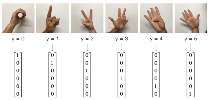
输出一张样例图片预览。
# Example of a picture
index = 6
plt.imshow(X_train_orig[index])
print("y = " + str(np.squeeze(Y_train_orig[:, index])))

数据预处理。将输入图像像素除以255进行归一化,将标签数据扩充为$one\_hot$编码,并且查看数据规模。
X_train = X_train_orig / 255.
X_test = X_test_orig / 255.
Y_train = convert_to_one_hot(Y_train_orig, 6).T
Y_test = convert_to_one_hot(Y_test_orig, 6).T
print("number of training examples = " + str(X_train.shape[0]))
print("number of test examples = " + str(X_test.shape[0]))
print("X_train shape: " + str(X_train.shape))
print("Y_train shape: " + str(Y_train.shape))
print("X_test shape: " + str(X_test.shape))
print("Y_test shape: " + str(Y_test.shape))
conv_layers = {}
Result:
number of training examples = 1080
number of test examples = 120
X_train shape: (1080, 64, 64, 3)
Y_train shape: (1080, 6)
X_test shape: (120, 64, 64, 3)
Y_test shape: (120, 6)
1.1 - Create placeholders
# GRADED FUNCTION: create_placeholders

def create_placeholders(n_H0, n_W0, n_C0, n_y):
    """
    Creates the placeholders for the tensorflow session.

    Arguments:
    n_H0 -- scalar, height of an input image
    n_W0 -- scalar, width of an input image
    n_C0 -- scalar, number of channels of the input
    n_y -- scalar, number of classes

    Returns:
    X -- placeholder for the data input, of shape [None, n_H0, n_W0, n_C0] and dtype "float"
    Y -- placeholder for the input labels, of shape [None, n_y] and dtype "float"
    """

    ### START CODE HERE ### (≈2 lines)
   # tf.placeholder第一个参数为类型,第二个参数位数据规模,可通过name参数指定变量名
    X = tf.placeholder(tf.float32, [None, n_H0, n_W0, n_C0])
    Y = tf.placeholder(tf.float32, [None, n_y])
    ### END CODE HERE ###

    return X, Y
X, Y = create_placeholders(64, 64, 3, 6)
print ("X = " + str(X))
print ("Y = " + str(Y))
Result:
X = Tensor("Placeholder_2:0", shape=(?, 64, 64, 3), dtype=float32)
Y = Tensor("Placeholder_3:0", shape=(?, 6), dtype=float32)
1.2 - Initialize parameters
通过$tf.contrib.layers.xavier\_initializer(seed=0)$初始化权重/过滤器/卷积核$W_1$和$W_2$,不用关心$bias\_variables$的初始化,因为TensorFlow方法会帮助我们做这件事,所以我们只需要初始化卷积方法的卷积核。TensorFlow也会自动初始化全连接层的参数。
使用TensorFlow初始化参数有如下语法:
W = tf.get_variable("W", [1,2,3,4], initializer = ...)
# GRADED FUNCTION: initialize_parameters

def initialize_parameters():
    """
    Initializes weight parameters to build a neural network with tensorflow. The shapes are:
                        W1 : [4, 4, 3, 8]
                        W2 : [2, 2, 8, 16]
    Returns:
    parameters -- a dictionary of tensors containing W1, W2
    """

    tf.set_random_seed(1)                              # so that your "random" numbers match ours

    ### START CODE HERE ### (approx. 2 lines of code)
    W1 = tf.get_variable("W1", [4, 4, 3, 8], initializer=tf.contrib.layers.xavier_initializer(seed=0))
    W2 = tf.get_variable("W2", [2, 2, 8, 16], initializer=tf.contrib.layers.xavier_initializer(seed=0))
    ### END CODE HERE ###

    parameters = {"W1": W1,
                  "W2": W2}

    return parameters
tf.reset_default_graph()
with tf.Session() as sess_test:
    parameters = initialize_parameters()
    init = tf.global_variables_initializer()
    sess_test.run(init)
    print("W1 = " + str(parameters["W1"].eval()[1,1,1]))
    print("W2 = " + str(parameters["W2"].eval()[1,1,1]))
Result:
W1 = [ 0.00131723  0.14176141 -0.04434952  0.09197326  0.14984085 -0.03514394
 -0.06847463  0.05245192]
W2 = [-0.08566415  0.17750949  0.11974221  0.16773748 -0.0830943  -0.08058
 -0.00577033 -0.14643836  0.24162132 -0.05857408 -0.19055021  0.1345228
 -0.22779644 -0.1601823  -0.16117483 -0.10286498]
1.3 - Forward propagation
在TensorFlow中,可以通过如下一些函数(语法)实现前向传播。
tf.nn.conv2d(X,W1, strides = [1,s,s,1], padding = 'SAME')
tf.nn.max_pool(A, ksize = [1,f,f,1], strides = [1,s,s,1], padding = 'SAME')
tf.nn.relu(Z1)
tf.contrib.layers.flatten(P)
tf.contrib.layers.fully_connected(F, num_outputs)
注意到,使用$tf.contrib.layers.fully\_connected$将会自动初始化全连接层的参数(权重),并且在训练模型的时候训练参数。因此我们无需初始化其参数。
实现方法$forward_propagation$,使其构造模型:CONV2D -> RELU -> MAXPOOL -> CONV2D -> RELU -> MAXPOOL -> FLATTEN -> FULLYCONNECTED。
# GRADED FUNCTION: forward_propagation

def forward_propagation(X, parameters):
    """
    Implements the forward propagation for the model:
    CONV2D -> RELU -> MAXPOOL -> CONV2D -> RELU -> MAXPOOL -> FLATTEN -> FULLYCONNECTED

    Arguments:
    X -- input dataset placeholder, of shape (input size, number of examples)
    parameters -- python dictionary containing your parameters "W1", "W2"
                  the shapes are given in initialize_parameters

    Returns:
    Z3 -- the output of the last LINEAR unit
    """

    # Retrieve the parameters from the dictionary "parameters"
    W1 = parameters['W1']
    W2 = parameters['W2']

    ### START CODE HERE ###
    # CONV2D: stride of 1, padding 'SAME'
    Z1 = tf.nn.conv2d(X, W1, strides=[1, 1, 1, 1], padding="SAME")
    # RELU
    A1 = tf.nn.relu(Z1)
    # MAXPOOL: window 8x8, sride 8, padding 'SAME'
    P1 = tf.nn.max_pool(A1, ksize=[1, 8, 8, 1], strides=[1, 8, 8, 1], padding="SAME")
    # CONV2D: filters W2, stride 1, padding 'SAME'
    Z2 = tf.nn.conv2d(P1, W2, strides=[1, 1, 1, 1], padding="SAME")
    # RELU
    A2 = tf.nn.relu(Z2)
    # MAXPOOL: window 4x4, stride 4, padding 'SAME'
    P2 = tf.nn.max_pool(A2, ksize=[1, 4, 4, 1], strides=[1, 4, 4, 1], padding="SAME")
    # FLATTEN
    P2 = tf.contrib.layers.flatten(P2)
    # FULLY-CONNECTED without non-linear activation function (not not call softmax).
    # 6 neurons in output layer. Hint: one of the arguments should be "activation_fn=None"
    Z3 = tf.contrib.layers.fully_connected(P2, 6, activation_fn=None)
    ### END CODE HERE ###

    return Z3
tf.reset_default_graph()

with tf.Session() as sess:
    np.random.seed(1)
    X, Y = create_placeholders(64, 64, 3, 6)
    parameters = initialize_parameters()
    Z3 = forward_propagation(X, parameters)
    init = tf.global_variables_initializer()
    sess.run(init)
    a = sess.run(Z3, {X: np.random.randn(2,64,64,3), Y: np.random.randn(2,6)})
    print("Z3 = " + str(a))
Result:
Z3 = [[ 1.44169843 -0.24909666  5.45049906 -0.26189619 -0.20669907  1.36546707]
 [ 1.40708458 -0.02573211  5.08928013 -0.48669922 -0.40940708  1.26248586]]
1.3 - Compute cost
# GRADED FUNCTION: compute_cost

def compute_cost(Z3, Y):
    """
    Computes the cost

    Arguments:
    Z3 -- output of forward propagation (output of the last LINEAR unit), of shape (6, number of examples)
    Y -- "true" labels vector placeholder, same shape as Z3

    Returns:
    cost - Tensor of the cost function
    """

    ### START CODE HERE ### (1 line of code)
    cost = tf.reduce_mean(tf.nn.softmax_cross_entropy_with_logits(logits=Z3, labels=Y))
    ### END CODE HERE ###

    return cost
tf.reset_default_graph()

with tf.Session() as sess:
    np.random.seed(1)
    X, Y = create_placeholders(64, 64, 3, 6)
    parameters = initialize_parameters()
    Z3 = forward_propagation(X, parameters)
    cost = compute_cost(Z3, Y)
    init = tf.global_variables_initializer()
    sess.run(init)
    a = sess.run(cost, {X: np.random.randn(4,64,64,3), Y: np.random.randn(4,6)})
    print("cost = " + str(a))
Result:
cost = 4.66487
1.4 - Model
整合上面实现了的有用的方法去构建一个模型在SIGNS数据集上进行训练。
将有几个步骤:
* 1 create placeholders
* 2 initialize parameters
* 3 forward propagate
* 4 compute the cost
* 5 create an optimizer
最后,创建一个$session$然后循环$num\_epochs$,每一次获得一个$mini-batches$并且通过模型预测出结果计算损失并且优化他们。
# GRADED FUNCTION: model

def model(X_train, Y_train, X_test, Y_test, learning_rate = 0.009,
          num_epochs = 100, minibatch_size = 64, print_cost = True):
    """
    Implements a three-layer ConvNet in Tensorflow:
    CONV2D -> RELU -> MAXPOOL -> CONV2D -> RELU -> MAXPOOL -> FLATTEN -> FULLYCONNECTED

    Arguments:
    X_train -- training set, of shape (None, 64, 64, 3)
    Y_train -- test set, of shape (None, n_y = 6)
    X_test -- training set, of shape (None, 64, 64, 3)
    Y_test -- test set, of shape (None, n_y = 6)
    learning_rate -- learning rate of the optimization
    num_epochs -- number of epochs of the optimization loop
    minibatch_size -- size of a minibatch
    print_cost -- True to print the cost every 100 epochs

    Returns:
    train_accuracy -- real number, accuracy on the train set (X_train)
    test_accuracy -- real number, testing accuracy on the test set (X_test)
    parameters -- parameters learnt by the model. They can then be used to predict.
    """

    ops.reset_default_graph()                         # to be able to rerun the model without overwriting tf variables
    tf.set_random_seed(1)                             # to keep results consistent (tensorflow seed)
    seed = 3                                          # to keep results consistent (numpy seed)
    (m, n_H0, n_W0, n_C0) = X_train.shape
    n_y = Y_train.shape[1]
    costs = []                                        # To keep track of the cost

    # Create Placeholders of the correct shape
    ### START CODE HERE ### (1 line)
   # 1 create placeholders
    X, Y = create_placeholders(n_H0, n_W0, n_C0, n_y)
    ### END CODE HERE ###

    # Initialize parameters
    ### START CODE HERE ### (1 line)
   # 2 initialize parameters
    parameters = initialize_parameters()
    ### END CODE HERE ###

    # Forward propagation: Build the forward propagation in the tensorflow graph
    ### START CODE HERE ### (1 line)
   # 3 forward propagate
    Z3 = forward_propagation(X, parameters)
    ### END CODE HERE ###

    # Cost function: Add cost function to tensorflow graph
    ### START CODE HERE ### (1 line)
   # 4 compute the cost
    cost = compute_cost(Z3, Y)
    ### END CODE HERE ###

    # Backpropagation: Define the tensorflow optimizer. Use an AdamOptimizer that minimizes the cost.
    ### START CODE HERE ### (1 line)
   # 5 create an optimizer
    optimizer = tf.train.AdamOptimizer(learning_rate).minimize(cost)
    ### END CODE HERE ###

    # Initialize all the variables globally
   # 初始化全部变量
    init = tf.global_variables_initializer()

    # Start the session to compute the tensorflow graph
   # 创建一个会话,并开始执行
    with tf.Session() as sess:

        # Run the initialization
        sess.run(init)

        # Do the training loop
     # 训练num_epoches轮
        for epoch in range(num_epochs):

            minibatch_cost = 0. # 保存当前mini_batch的cost
            num_minibatches = int(m / minibatch_size) # number of minibatches of size minibatch_size in the train set
            seed = seed + 1
            minibatches = random_mini_batches(X_train, Y_train, minibatch_size, seed) # 随机从训练集中获取一个mini_batch

            for minibatch in minibatches: # 遍历mini_batch中的训练数据,计算损失

                # Select a minibatch
                (minibatch_X, minibatch_Y) = minibatch
                # IMPORTANT: The line that runs the graph on a minibatch.
                # Run the session to execute the optimizer and the cost, the feedict should contain a minibatch for (X,Y).
                ### START CODE HERE ### (1 line)
                _ , temp_cost = sess.run([optimizer, cost], feed_dict={X:minibatch_X, Y:minibatch_Y})
                ### END CODE HERE ###

                minibatch_cost += temp_cost / num_minibatches


            # Print the cost every epoch
            if print_cost == True and epoch % 5 == 0: # 每5轮输出一次当前损失值
                print ("Cost after epoch %i: %f" % (epoch, minibatch_cost))
            if print_cost == True and epoch % 1 == 0: # 取偶数轮数的损失值来画折线图
                costs.append(minibatch_cost)


        # plot the cost
     # 画出损失值折线图
        plt.plot(np.squeeze(costs))
        plt.ylabel('cost')
        plt.xlabel('iterations (per tens)')
        plt.title("Learning rate =" + str(learning_rate))
        plt.show()

        # Calculate the correct predictions
     # 计算预测准确率
        predict_op = tf.argmax(Z3, 1)
        correct_prediction = tf.equal(predict_op, tf.argmax(Y, 1))

        # Calculate accuracy on the test set
     # 计算训练集准确率以及测试集准确率并且打印出来
        accuracy = tf.reduce_mean(tf.cast(correct_prediction, "float"))
        print(accuracy)
        train_accuracy = accuracy.eval({X: X_train, Y: Y_train})
        test_accuracy = accuracy.eval({X: X_test, Y: Y_test})
        print("Train Accuracy:", train_accuracy)
        print("Test Accuracy:", test_accuracy)

        return train_accuracy, test_accuracy, parameters
_, _, parameters = model(X_train, Y_train, X_test, Y_test)

fname = "images/thumbs_up.jpg"
image = np.array(ndimage.imread(fname, flatten=False))
my_image = scipy.misc.imresize(image, size=(64,64))
plt.imshow(my_image)


 浙公网安备 33010602011771号