谣言检测（ACLR）《Detect Rumors in Microblog Posts for Low-Resource Domains via Adversarial Contrastive Learning》

论文信息

论文标题：Detect Rumors in Microblog Posts for Low-Resource Domains via Adversarial Contrastive Learning
论文作者：Hongzhan Lin, Jing Ma, Liangliang Chen, Zhiwei Yang, Mingfei Cheng, Guang Chen
论文来源：NAACL 2022
论文地址：download 
论文代码：download

1 Introduction

　　水文.....................，后续工作也是水文一篇。

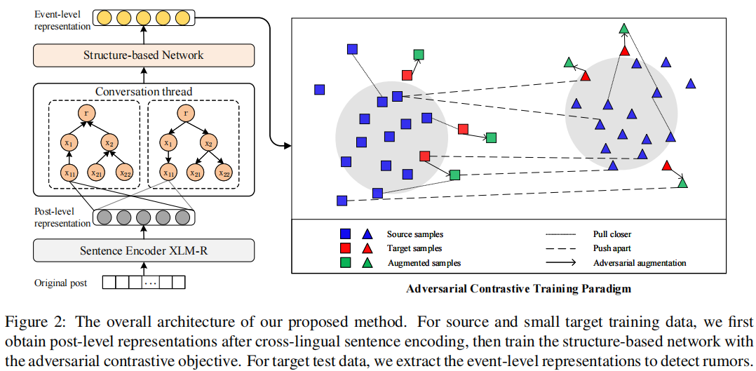
　　第一个提出一个全新的对抗性对比学习框架来研究社交媒体上的低资源谣言检测；

　　提出了监督对比学习用于不同领域和语言之间的结构特征适应，使用对抗攻击来增强对比范式中低资源数据的多样性；

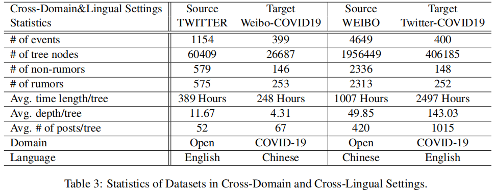
　　构建了两个具有传播树结构的 COVID-19 对应的低资源微博数据集（英文和中文）；

2 Problem Statement

　　In this work, we define the low-resource rumor detection task as: Given a well-resourced dataset as source, classify each event in the target lowre-source dataset as a rumor or not, where the source and target data are from different domains and/or languages. Specifically, we define a well-resourced source dataset for training as a set of events  $\mathcal{D}_{s}=\left\{C_{1}^{s}, C_{2}^{s}, \cdots, C_{M}^{s}\right\}$ , where  $M$  is the number of source events. Each event  $C^{s}=(y, c, \mathcal{T}(c))$  is a tuple representing a given claim  $c$  which is associated with a veracity label  $y \in\{  rumor, non-rumor  \}$ , and ideally all its relevant responsive microblog post in chronological order, i.e., $\mathcal{T}(c)=\left\{c, x_{1}^{s}, x_{2}^{s}, \cdots, x_{|C|}^{s}\right\}^{3}$ , where $|C|$ is the number of responsive tweets in the conversation thread. For the target dataset with low-resource domains and/or languages, we consider a much smaller dataset for training $\mathcal{D}_{t}=\left\{C_{1}^{t}, C_{2}^{t}, \cdots, C_{N}^{t}\right\}$ , where $N(N \ll M)$ is the number of target events and each $C^{t}= \left(y, c^{\prime}, \mathcal{T}\left(c^{\prime}\right)\right)$ has the similar composition structure of the source dataset.

　　We formulate the task of low-resource rumor detection as a supervised classification problem that trains a domain/language-agnostic classifier $f(\cdot)$ adapting the features learned from source datasets to that of the target events, that is, $f\left(C^{t} \mid \mathcal{D}_{s}\right) \rightarrow y$ . Note that although the tweets are notated sequentially, there are connections among them based on their responsive relationships. So most previous works represent the conversation thread as a tree structure .

3 Method

总体框架：

　　

3.1 Cross-lingual Sentence Encoder 

　　首先利用 XLM-RoBERTa（XLM-R）来获得句子表示：

　　　　$\bar{x}=X L M-R(\mathbf{x})$

　　本文使用 XLM-R 中 token <s> 标记的输出状态作为句子表示 $\bar{x}$。

　　使用上述过程可以得到 source event 和 target event 的特征矩阵 $X^{*}=\left[\bar{x}_{0}^{*}, \bar{x}_{1}^{*}, \bar{x}_{2}^{*}, \ldots, \bar{x}_{\left|X^{*}\right|-1}^{*}\right]^{\top} $，$* \in\{s, t\}$ ，其中 $X^{s} \in \mathbb{R}^{m \times d}$ 、$X^{t} \in \mathbb{R}^{n \times d}$。

代码：

tokenizer = XLMRobertaTokenizer.from_pretrained('xlm-roberta-base')
token_model = XLMRobertaModel.from_pretrained('xlm-roberta-base')
def str2vec(str):
    inputs = tokenizer(str, return_tensors="pt")
    outputs = token_model(**inputs)
    last_hidden_states = outputs.last_hidden_state #torch.Size([1, sen_len, 768])
    sen_len=int(last_hidden_states.size()[-2])-2
    # word_vec= last_hidden_states.squeeze(0)[1:-1]  #drop out the [CLS] and [SEP]
    word_vec = last_hidden_states.squeeze(0)[0]   #sentece_vector
    return word_vec.tolist(), sen_len

3.2 Propagation Structure Representation

Top-Down GCN、Bottom-Up GCN

　　　　$H^{(l+1)}=\operatorname{Re} L U\left(\hat{\mathbf{A}} \cdot H^{(l)} \cdot W^{(l)}\right)$

　　　　$\hat{\mathbf{A}}=\mathbf{D}^{-1 / 2} \mathbf{A} \mathbf{D}^{-1 / 2}$

The Overall Model

　　最后，通过均值池将 $H_{TD}$ 和 $H_{BU}$ 连接起来，以共同捕获自上而向下和自下而上两种树中表达的观点：

　　　　$o=\text { mean-pooling }\left(\left[H_{T D} ; H_{B U}\right]\right)\in\mathbb{R}^{2 d^{(L)}}$

3.3 Contrastive Training

　　给定源域数据，使用上述平均池化得到的 $o_{i}^{s}$ ，放入 softmax 做谣言分类，使用 CE loss ：

　　　　$\mathcal{L}_{C E}^{s}=-\frac{1}{N^{s}} \sum\limits _{i=1}^{N^{s}} \log \left(p_{i}\right)$

　　其中，$N^{s}$ 是 Batch 中的源域数据，$p_{i}$ 是 正确预测的概率；

　　为了使源事件中的谣言表示更具指示性，提出一个监督对比学习目标，以聚集同一类，并分离不同类别的样本：

　　　　$\mathcal{L}_{S C L}^{s}=-\frac{1}{N^{s}} \sum\limits_{i=1}^{N^{s}} \frac{1}{N_{y_{i}^{s}}-1} \sum\limits_{j=1}^{N^{s}} \mathbb{1}_{[i \neq j]} \mathbb{1}_{\left[y_{i}^{s}=y_{j}^{s}\right]} \log \frac{\exp \left(\operatorname{sim}\left(o_{i}^{s}, o_{j}^{s}\right) / \tau\right)}{\sum\limits _{k=1}^{N^{s}} \mathbb{1}_{[i \neq k]} \exp \left(\operatorname{sim}\left(o_{i}^{s}, o_{k}^{s}\right) / \tau\right)}$

　　其中，$ N_{y_{i}^{s}}$ 是 source 数据中拥有一样标签 $y_{i}^{s} $ 的数量。 

　　为充分利用 target 数据，通过对比表学习将源域数据和目标域数据有相同标签的样本拉近：

　　　　$\mathcal{L}_{S C L}^{t}=-\frac{1}{N^{t}} \sum\limits_{i=1}^{N^{t}} \frac{1}{N_{y_{i}^{t}}} \sum\limits_{j=1}^{N^{s}} \mathbb{1}_{\left[y_{i}^{t}=y_{j}^{s}\right]} \log \frac{\exp \left(\operatorname{sim}\left(o_{i}^{t}, o_{j}^{s}\right) / \tau\right)}{\sum\limits_{k=1}^{N^{s}} \exp \left(\operatorname{sim}\left(o_{i}^{t}, o_{k}^{s}\right) / \tau\right)}$

3.4 Adversarial Data Augmentation

　　在本节中，引入对抗性攻击，在事件级潜在空间生成伪目标样本，以增加模型视图的多样性，以实现对比学习方式的鲁棒性。具体来说，我们应用Fast Gradient Value 将最坏情况扰动近似为事件级表示的噪声向量：

　　　　$\tilde{\boldsymbol{o}}_{n o i s e}^{t}=\epsilon \frac{g}{\|g\|} ; \text { where } g=\nabla_{o^{t}} \mathcal{L}_{C E}^{t}$

　　其中，梯度 $g$ 为目标样本的分类损失 $\mathcal{L}_{C E}^{t}$ 的一阶差分，即快速增加分类损失的方向。我们执行归一化，并使用一个小的 $\epsilon$，以确保近似是合理的。

　　最后，我们可以在潜在空间中获得伪增强样本 $ o_{a d v}^{t}= o^{t}+\tilde{\boldsymbol{o}}_{\text {noise }}^{t} $ 来增强我们的模型。

3.5 Model Training

　　联合训练：

　　　　$\mathcal{L}^{*}=(1-\alpha) \mathcal{L}_{C E}^{*}+\alpha \mathcal{L}_{S C L}^{*} ; * \in\{s, t\}$

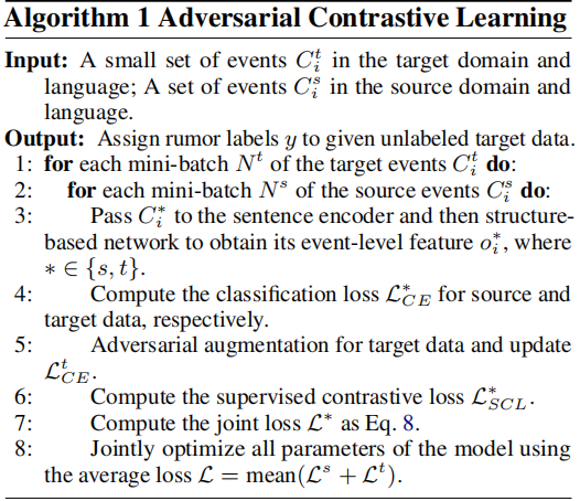
　　代码：源域对比损失+源域交叉熵损失+交叉域对比损失+目标域交叉熵损失+交叉域对比损失（噪声）+目标域分类损失（噪声）

class Net(torch.nn.Module):
    def __init__(self,in_feats,hid_feats,out_feats,temperature):
        super(Net, self).__init__()
        self.TDrumorGCN = TDrumorGCN(in_feats, hid_feats, out_feats)
        self.BUrumorGCN = BUrumorGCN(in_feats, hid_feats, out_feats)
        self.fc=torch.nn.Linear((out_feats+hid_feats)*2,2)
        self.scl = SCL(temperature)

    def forward(self, data, twitter_data=None):
        if twitter_data is None:
            x = data.x

            TD_x = self.TDrumorGCN(x, data)
            BU_x = self.BUrumorGCN(x, data)
            x = torch.cat((BU_x, TD_x), 1)
            x = self.fc(x)
            x = F.log_softmax(x, dim=1)
            return x
        else:
            t = twitter_data.x
            TD_t = self.TDrumorGCN(t, twitter_data)
            BU_t = self.BUrumorGCN(t, twitter_data)
            t_ = torch.cat((BU_t, TD_t), 1)
            twitter_scloss = self.scl(t_,t_, twitter_data.y)                #源域对比损失
            t = self.fc(t_)
            t = F.log_softmax(t, dim=1)
            twitter_CEloss = F.nll_loss(t, twitter_data.y)                  #源域交叉熵损失

            # COVID 数据集====================
            x=data.x
            TD_x = self.TDrumorGCN(x, data)
            BU_x = self.BUrumorGCN(x, data)
            x_ = torch.cat((BU_x,TD_x), 1) #bs, (out_feats+hid_feats)*2
            weibocovid19_scloss = self.scl(x_,t_, data.y, twitter_data.y)   #交叉域对比损失

            x = self.fc(x_)
            x = F.log_softmax(x, dim=1)
            weibocovid19_CEloss = F.nll_loss(x, data.y)                     #目标域交叉熵损失

            # normal_loss= 0.5*(0.7*twitter_CEloss+0.3*twitter_scloss)+ 0.5*(0.7*weibocovid19_CEloss+0.3*weibocovid19_scloss)
            x_.retain_grad()  # we need to get gradient w.r.t low-resource embeddings
            weibocovid19_CEloss.backward(retain_graph=True)
            unnormalized_noise = x_.grad.detach_()
            for p in self.parameters():
                if p.grad is not None:
                    p.grad.detach_()
                    p.grad.zero_()
            norm = unnormalized_noise.norm(p=2, dim=-1)
            normalized_noise = unnormalized_noise / (norm.unsqueeze(dim=-1) + 1e-10)  # add 1e-10 to avoid Nan
            noise_norm = 1.5
            alp = 0.5
            target_noise = noise_norm * normalized_noise
            noise_x_ = x_ + target_noise
            noise_scloss = self.scl(noise_x_, t_, data.y, twitter_data.y)                 #交叉域对比损失，（噪声）
            noise_CEloss = F.nll_loss(F.log_softmax(self.fc(noise_x_), dim=1), data.y)    #目标域分类损失（噪声）
            noise_loss = (1-alp) * noise_CEloss + alp * noise_scloss
            total_loss = (((1-alp) * twitter_CEloss + alp * twitter_scloss) + ((1-alp) * weibocovid19_CEloss + alp * weibocovid19_scloss) + noise_loss) / 3
            return total_loss, x

　　算法总结：

　　

4 Experiments

数据集

　　

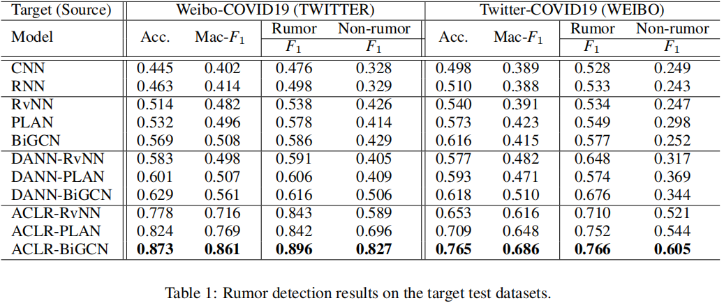
谣言检测性能

　　

消融实验

　　

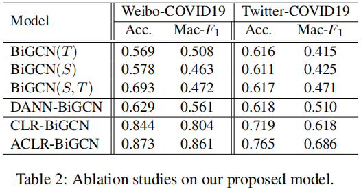
• We observe that the model performs best if pre-trained on source data and then fine-tuned on target training data (i.e., BiGCN(S,T)), compared with the poor performance when trained on either minor labeled target data only (i.e., BiGCN(T)) or well-resourced source data (i.e., BiGCN(S)).
• In the second group, the DANN-based model makes better use of the source data to extract domain-agnostic features, which further leads to performance improvement.
• Our proposed contrastive learning approach CLR without adversarial augmentation mechanism, has already achieved outstanding performance compared with other baselines, which illustrates its effectiveness on domain and language adaptation. We further notice that our ACLR-BiGCN consistently outperforms all baselines and improves the prediction performance of CLR-BiGCN, suggesting that training model together with adversarial augmentation on target data provide positive guidance for more accurate rumor predictions, especially in low-resource regimes.

早期检测

　　

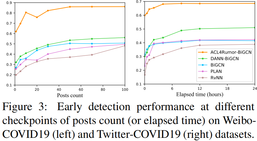
• Firstly, we observe that our proposed ACLR-based approach outperforms other counterparts and baselines throughout  the whole lifecycle, and reaches a relatively high Macro F1 score at a very early period after the initial broadcast.
• One interesting phenomenon is that the early performance of some methods may fluctuate more or less. It is because with the propagation of the claim there is more semantic and structural information but the noisy information is increased simultaneously.

特征可视化

　　Figure 4 显示了在BiGCN（left）和ACLR-BiGCN（right）上学习到的目标事件级特征的 PCA 可视化分析。

　　

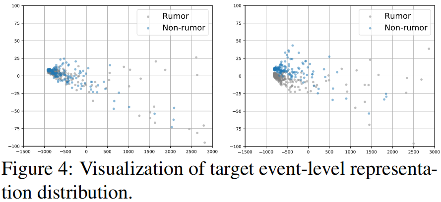
• due to the lack of sufficient training data, the features extracted with the traditional training paradigm are entangled, making it difficult to detect rumors in low-resource regimes;
• our ACLRbased approach learns more discriminative representations to improve low-resource rumor classifi- cation, reaffirming that our training paradigm can effectively transfer knowledge to bridge the gap between source and target data distribution resulting from different domains and languages.

5 Conclusion and Future Work

　　在本文中，我们提出了一种新的对抗性对比学习框架，通过将从资源充足的数据中学习到的特征适应于低资源破坏事件的特征，来弥补谣言检测的低资源缺口。在两个真实基准上的结果证实了我们的模型在低资源谣言检测任务中的优势。在我们未来的工作中，我们计划收集和应用我们的模型在其他领域和少数民族语言。