论文信息
论文标题:Graph Auto-Encoder via Neighborhood Wasserstein Reconstruction
论文作者:Shaked Brody, Uri Alon, Eran Yahav
论文来源:2022,ICLR
论文地址:download
论文代码:download
1 Abstract
提出了一种新的图自编码器,其中 Encoder 为普通的 GAE,而 Decoder 实现了特征重建、度重建,以及一种基于 2-Wasserstein distance 的邻居重建。
2 Introduction
两种典型的 GAE :
-
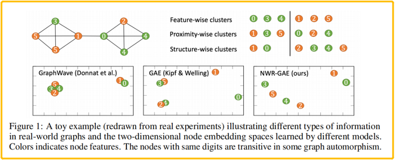
- GAE(Kipf & Welling, 2016)使用简单的重建链接结构,导致无法区分像 (2, 4) 和 (3, 5)这样的点;
- GraphWave (Donnat et al., 2018) 面向结构的嵌入模型不考虑节点特征和空间接近度,无法区分像 (0, 1), (2, 4) 和 (3,5) 的节点对;
本文提出的 新框架为 Neighborhood Wasserstein Reconstruction Graph Auto-Encoder (NWR-GAE),将重构损失分解为三个部分,即 节点度、邻居表示分布和节点特征。
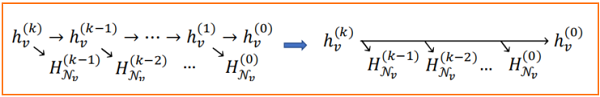
其中最重要的是重建邻居分布,由于在 消息传递后,在节点 的表示中编码的信息来源本质上来自于 的 邻域(Fig.2)。因此,节点 的良好表示应该捕获其 跳邻域中所有节点的特征信息,这与下游任务是无关的。

考虑两个分布之间的距离:当两个分布有非重叠的部分时, 散度家族存在非连续的问题。
Suppose we have two probability distributions, and :
When :
But when , two distributions are fully overlapped:

可以使用 最优传输 OT 的 2-Wasserstein distance 衡量两个分布之间的距离,在这里,给出一个基于 2-Wasserstein distance 的常用的 OT 损失:
Definition 2.1. Let , denote two probability distributions with finite second moment defined on . The 2-Wasserstein distance between and defined on , is the solution to the optimal mass transportation problem with transport cost (Villani, 2008):
where contains all joint distributions of with marginals and respectively.
3 Methods
预先定义 :
-
- Encoder:
- Decoder:
Encoder 可以是任何基于消息传递的 GNNs,Decoder 可以分成三部分:
3.1 Neighborhood peconstruction principle
本文只考虑 1-hop 邻域重建。用 代表 初始特征矩阵,对于每个节点 被 GNN Enocoder 编码后 ,其节点表示 从 及其邻居表示 。本文主要目的是重构来自 和 的信息,因此有
其中, 定义了重建损失, 可分为两部分,分别测量自 特征重建 和 邻域重建:
对于特征重建,及其特征重建损失函数 :
代码中:
feature_losses = self.feature_loss_func(h0, self.feature_decoder(gij))
其实 h0 代表原始特征矩阵 ,而 gij 是经过四层的 GCN encoder 得到的隐表示,然后使用一个 FNN 的 feature_decoder 将 gij 的维度映射成和 一样大。
被分为度重建和 邻居重建,对于节点 ,邻域信息被表示为 i.i.d .的经验实现从 中采样 元素,其中 。具体来说,采用
Generalizing to k-hop neighborhood reconstruction
本文期望 直接重构 。具体来说,对于每个节点 ,使用重构损失
其中 是解码初始特征, 是度解码,, 是解码 层邻域表示分布 。 和 为非负性超参数。因此, 跳邻域重建的全部目标是
其中, 包括 个GNN层, 在 中定义。
3.2 Decoding distributions——Decoders
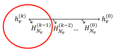
Note :上述图说的其实是使用 第 的节点 的节点表示重建邻域 。
上代码悟:

self.m = torch.distributions.Normal(torch.zeros(sample_size, hidden_dim),torch.ones(sample_size, hidden_dim))
self.mlp_mean = nn.Linear(hidden_dim, hidden_dim)
self.mlp_sigma = nn.Linear(hidden_dim, hidden_dim)

sampled_embeddings_list, mark_len_list = self.sample_neighbors(neighbor_indexes, neighbor_dict, to_layer)    #从第 k-1 层采样节点的5个邻居节点,未满五个的使用 0 填充特征矩阵
for i, neighbor_embeddings1 in enumerate(sampled_embeddings_list):
    # Generating h^k_v, reparameterization trick
    index = neighbor_indexes[i]
    mask_len1 = mark_len_list[i]
    mean = from_layer[index].repeat(self.sample_size, 1)      #[5,512]   ,获取第 k 层的 节点 v 的表示
    mean = self.mlp_mean(mean)                                #[5,512]   ,线性变换
    sigma = from_layer[index].repeat(self.sample_size, 1)   #[5,512]   ,获取第 k 层的 节点 v 的表示
    sigma = self.mlp_sigma(sigma)                        #[5,512]   ,线性变换
    std_z = self.m.sample().to(device)                  # [5,512]  ,每个元素为均值为0,标准差为1 的正态分布生成
    var = mean + sigma.exp() * std_z                  # [5,512]      正态分布处理生成的邻居表示集合
    nhij = FNN_generator(var, device)                 #[5,512]  ,前馈神经网络线性变换
    generated_neighbors = nhij
接着就去计算 节点 的邻域 和生成的邻域之间的 2-Wasserstein distance ,这里的代码我没看懂,好难过啊。
3.3 Further discussion-Decoders 、 and Encoder
3.3.1 degree_decoder
重构节点度的解码器 是一个 FNN+ReLU 激活函数,使其值非负。
度解码器代码:


self.degree_decoder = FNN(hidden_dim, hidden_dim, 1, 4)

# FNN
class FNN(nn.Module):
    def __init__(self, in_features, hidden, out_features, layer_num):
        super(FNN, self).__init__()
        self.linear1 = MLP(layer_num, in_features, hidden, out_features)
        self.linear2 = nn.Linear(out_features, out_features)
    def forward(self, embedding):
        x = self.linear1(embedding)
        x = self.linear2(F.relu(x))
        return x

def degree_decoding(self, node_embeddings):
    degree_logits = F.relu(self.degree_decoder(node_embeddings))
    return degree_logits
度重构采用的损失函数 MSE loss:
self.degree_loss_func = nn.MSELoss()
3.3.2 feature_decoder
重构初始特征 的解码器 是一个 FNN。
特征解码器代码:
self.feature_decoder = FNN(hidden_dim, hidden_dim, in_dim, 3)

# FNN
class FNN(nn.Module):
    def __init__(self, in_features, hidden, out_features, layer_num):
        super(FNN, self).__init__()
        self.linear1 = MLP(layer_num, in_features, hidden, out_features)
        self.linear2 = nn.Linear(out_features, out_features)
    def forward(self, embedding):
        x = self.linear1(embedding)
        x = self.linear2(F.relu(x))
        return x
特征重构采用的损失函数 MSE loss:
self.feature_loss_func = nn.MSELoss()
3.3.3 Encoder
Encoder 可以为 GINConv、GraphConv、SAGEConv layer, 考虑到本实验堆叠了多层 GNNs layer,所以很容易造成过平滑,故,这里采用 PairNorm 缓解过平滑存在的问题。
Encoder 代码:
if GNN_name == "GCN":
    self.graphconv1 = GraphConv(in_dim, hidden_dim)            #[1433,512]
    self.graphconv2 = GraphConv(hidden_dim, hidden_dim)         #[512,512]
    self.graphconv3 = GraphConv(hidden_dim, hidden_dim)        #[512,512]
    self.graphconv4 = GraphConv(hidden_dim, hidden_dim)       #[512,512]

self.norm = PairNorm(norm_mode, norm_scale)

def forward_encoder(self, g, h):
    # K-layer Encoder
    # Apply graph convolution and activation, pair-norm to avoid trivial solution
    h0 = h
    l1 = self.graphconv1(g, h0)
    l1_norm = torch.relu(self.norm(l1))
    l2 = self.graphconv2(g, l1_norm)
    l2_norm = torch.relu(self.norm(l2))
    l3 = self.graphconv3(g, l2)
    l3_norm = torch.relu(l3)
    l4 = self.graphconv4(g, l1_norm) # 5 layers
    return l4, l3_norm, l2_norm, l1_norm, h0

class PairNorm(nn.Module):
    ...
    def forward(self, x):
        if self.mode == 'None':
            return x
        col_mean = x.mean(dim=0)
        if self.mode == 'PN':
            x = x - col_mean
            rownorm_mean = (1e-6 + x.pow(2).sum(dim=1).mean()).sqrt()
            x = self.scale * x / rownorm_mean
        if self.mode == 'PN-SI':
            x = x - col_mean
            rownorm_individual = (1e-6 + x.pow(2).sum(dim=1, keepdim=True)).sqrt()
            x = self.scale * x / rownorm_individual
        if self.mode == 'PN-SCS':
            rownorm_individual = (1e-6 + x.pow(2).sum(dim=1, keepdim=True)).sqrt()
            x = self.scale * x / rownorm_individual - col_mean
        return x
4 Experiments
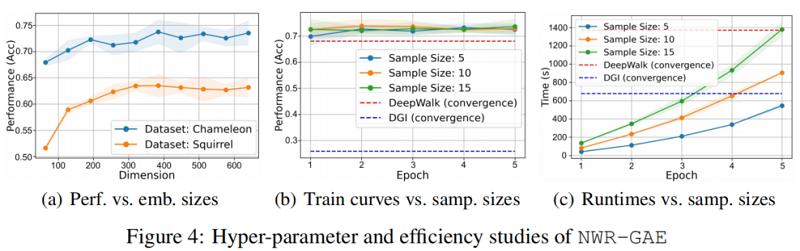
我们设计实验来评估 NWR-GAE,重点关注以下研究问题:RQ1:与最先进的无监督图嵌入基线相比,NWR-GAE在基于结构角色的合成数据集上表现如何?RQ2:NWR-GAE及其消融如何与不同类型的真实世界图形数据集上的基线进行比较?RQ3:嵌入尺寸 和采样尺寸 等主要模型参数对NWR-GAE的影响是什么?
4.1 Experimental setup
4.1.1 Datasets
Synthetic datasets
4.1.2 Baselines
1) Random walk based (DeepWalk, node2vec)
2) Structural role based (RoleX, struc2vec, GraphWave)
3) Graph auto-encoder based (GAE, VGAE, ARGVA)
4) Contrastive learning based (DGI, GraphCL, MVGRL)
4.1.3 Evaluation metrics
- Homogeneity: conditional entropy of ground-truth among predicting clusters.
- Completeness: ratio of nodes with the same ground-truth labels assigned to the same cluster.
- Silhouette score: intra-cluster distance vs. inter-cluster distance.
4.2 Performance on synthetic datasets(RQ1)

4.3 Performance on real-world datasets(RQ2)
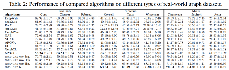
4.4 In-depth analysis of NWR-GAE
5 Conclusion
在这项工作中,我们解决了现有的无监督图表示方法的局限性,并提出了第一个能够正确地捕获图中节点的接近性、结构和特征信息的模型,并在低维嵌入空间中对其进行区分编码的模型。该模型在合成和真实基准数据集上进行了广泛的测试,结果有力地支持了其声称的优势。由于它是通用的,有效的,而且在概念上也很容易理解,我们相信它有潜力作为无监督图表示学习的实际方法。在未来,它将有望看到其在不同领域的应用研究,以及仔细分析其鲁棒性和隐私性等潜在问题。
因上求缘,果上努力~~~~ 作者:别关注我了,私信我吧,转载请注明原文链接:https://www.cnblogs.com/BlairGrowing/p/16599030.html


【推荐】国内首个AI IDE,深度理解中文开发场景,立即下载体验Trae
【推荐】编程新体验,更懂你的AI,立即体验豆包MarsCode编程助手
【推荐】抖音旗下AI助手豆包,你的智能百科全书,全免费不限次数
【推荐】轻量又高性能的 SSH 工具 IShell:AI 加持,快人一步
· 震惊!C++程序真的从main开始吗?99%的程序员都答错了
· winform 绘制太阳,地球,月球 运作规律
· 【硬核科普】Trae如何「偷看」你的代码?零基础破解AI编程运行原理
· 上周热点回顾(3.3-3.9)
· 超详细:普通电脑也行Windows部署deepseek R1训练数据并当服务器共享给他人
2021-08-20 Alex网络结构
2020-08-20 451. 根据字符出现频率排序
2020-08-20 剑指 Offer 40. 最小的k个数
2020-08-20 list使用详解
2020-08-20 STL---priority_queue
2020-08-20 1046. 最后一块石头的重量