论文信息
论文标题:Self-Attention Graph Pooling
论文作者:Junhyun Lee, Inyeop Lee, Jaewoo Kang
论文来源:2019, ICML
论文地址:download
论文代码:download
1 Preamble
对图使用下采样 downsampling (pooling)。
2 Introduction
图池化三种类型:
-
- Topology based pooling;
-
Global pooling;
- Hierarchical pooling;
关于 Hierarchical pooling 聚类分配矩阵:
其中, , 代表 第 层的节点数量。
gPool 取得了与 DiffPool 相当的性能,gPool 的存储复杂度为 ,而 DiffPool 需要 ,其中 、 和 分别表示顶点、边和池化率。gPool 使用一个可学习的向量 来计算投影分数,然后使用这些分数来选择排名靠前的节点。投影得分由 与所有节点的特征之间的点积得到。这些分数表示可以保留的节点的信息量。下面的公式大致描述了 gPool 中的池化过程:
3 Method
框架如下:
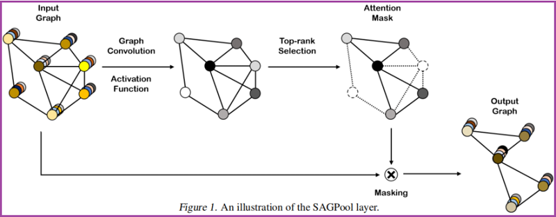
3.1 Self-Attention Graph Pooling
Self-attention mask
本文使用图卷积来获得自注意分数:
其中:
-
- 自注意得分 ;
- 邻接矩阵 ;
- 注意力参数矩阵 ;
- 特征矩阵 ;
- 度矩阵 ;
保留部分重要节点:
基于自注意得分 ,保留前 个节点,其中 代表着池化率, 是 feature attention mask。
Graph pooling
获得新特征矩阵和邻接矩阵:
其中, 哈达玛积。
Variation of SAGPool
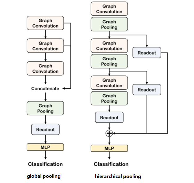
3.2 Model Architecture
本节用来验证模块的有效性。
Convolution layer
图卷积 GCN:
与 不同的是, 。
Readout layer
根据 JK-net architecture 的思想:
其中:
- 代表着节点的个数;
- 代表着第 个节点的特征向量;
代码:
x = F.relu(self.conv1(x, edge_index))
x, edge_index, _, batch, _ = self.pool1(x, edge_index, None, batch)
x1 = torch.cat([global_max_pool(x, batch), global_mean_pool(x, batch)], dim=1)
即:平均池化和 最大池化进行拼接。
Global pooling architecture & Hierarchical pooling architecture
对比如下:
Model Code:

class Net(torch.nn.Module):
    def __init__(self, args):
        super(Net, self).__init__()
        self.args = args
        self.num_features = args.num_features
        self.nhid = args.nhid
        self.num_classes = args.num_classes
        self.pooling_ratio = args.pooling_ratio
        self.dropout_ratio = args.dropout_ratio

        self.conv1 = GCNConv(self.num_features, self.nhid)
        self.pool1 = SAGPool(self.nhid, ratio=self.pooling_ratio)
        self.conv2 = GCNConv(self.nhid, self.nhid)
        self.pool2 = SAGPool(self.nhid, ratio=self.pooling_ratio)
        self.conv3 = GCNConv(self.nhid, self.nhid)
        self.pool3 = SAGPool(self.nhid, ratio=self.pooling_ratio)

        self.lin1 = torch.nn.Linear(self.nhid * 2, self.nhid)
        self.lin2 = torch.nn.Linear(self.nhid, self.nhid // 2)
        self.lin3 = torch.nn.Linear(self.nhid // 2, self.num_classes)

    def forward(self, data):
        # 读取每个 batch 中的图数据
        x, edge_index, batch = data.x, data.edge_index, data.batch

        # 第一次做 Self-Attention Graph Pooling=======
        x = F.relu(self.conv1(x, edge_index))
        x, edge_index, _, batch, _ = self.pool1(x, edge_index, None, batch)
        # 第一次 Readout layer
        x1 = torch.cat([gmp(x, batch), gap(x, batch)], dim=1)

        # 第二次做 Self-Attention Graph Pooling=======
        x = F.relu(self.conv2(x, edge_index))
        x, edge_index, _, batch, _ = self.pool2(x, edge_index, None, batch)
        # 第二次 Readout layer
        x2 = torch.cat([gmp(x, batch), gap(x, batch)], dim=1)

        # 第三次做 Self-Attention Graph Pooling=======
        x = F.relu(self.conv3(x, edge_index))
        x, edge_index, _, batch, _ = self.pool3(x, edge_index, None, batch)
        # 第三次 Readout layer
        x3 = torch.cat([gmp(x, batch), gap(x, batch)], dim=1)

        # 跳跃连接
        x = x1 + x2 + x3

        # MLP
        x = F.relu(self.lin1(x))
        x = F.dropout(x, p=self.dropout_ratio, training=self.training)
        x = F.relu(self.lin2(x))
        x = F.log_softmax(self.lin3(x), dim=-1)
        return x
SAGPool Code:
class SAGPool(torch.nn.Module):
    def __init__(self,in_channels,ratio=0.8,Conv=GCNConv,non_linearity=torch.tanh):
        super(SAGPool,self).__init__()
        self.in_channels = in_channels
        self.ratio = ratio
        self.score_layer = Conv(in_channels,1)
        self.non_linearity = non_linearity
    def forward(self, x, edge_index, edge_attr=None, batch=None):
        if batch is None:
            batch = edge_index.new_zeros(x.size(0))

        #x = x.unsqueeze(-1) if x.dim() == 1 else x
        score = self.score_layer(x,edge_index).squeeze()
        perm = topk(score, self.ratio, batch)
        x = x[perm] * self.non_linearity(score[perm]).view(-1, 1)
        batch = batch[perm]
        edge_index, edge_attr = filter_adj(
            edge_index, edge_attr, perm, num_nodes=score.size(0))

        return x, edge_index, edge_attr, batch, perm
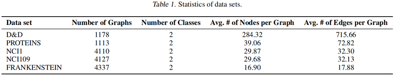
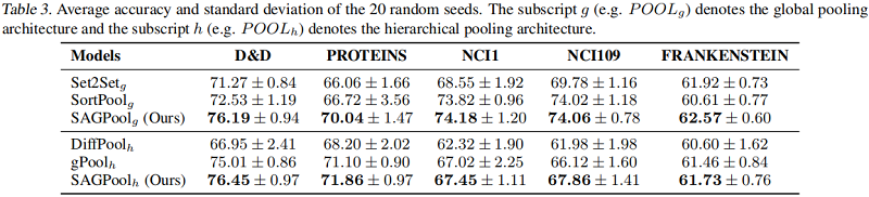
4 Experiments
数据集
基线实验
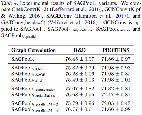
SAGPool 的变体
5 Conclusion
本文提出了一种基于自注意的SAGPool图池化方法。我们的方法具有以下特征:分层池、同时考虑节点特征和图拓扑、合理的复杂度和端到端表示学习。SAGPool使用一致数量的参数,而不管输入图的大小如何。我们工作的扩展可能包括使用可学习的池化比率来获得每个图的最优聚类大小,并研究每个池化层中多个注意掩模的影响,其中最终的表示可以通过聚合不同的层次表示来获得。
修改历史
2022-05-08 创建文章
2022-08-12 修订文章
因上求缘,果上努力~~~~ 作者:别关注我了,私信我吧,转载请注明原文链接:https://www.cnblogs.com/BlairGrowing/p/16230073.html


【推荐】国内首个AI IDE,深度理解中文开发场景,立即下载体验Trae
【推荐】编程新体验,更懂你的AI,立即体验豆包MarsCode编程助手
【推荐】抖音旗下AI助手豆包,你的智能百科全书,全免费不限次数
【推荐】轻量又高性能的 SSH 工具 IShell:AI 加持,快人一步
· 【自荐】一款简洁、开源的在线白板工具 Drawnix
· 没有Manus邀请码?试试免邀请码的MGX或者开源的OpenManus吧
· 无需6万激活码!GitHub神秘组织3小时极速复刻Manus,手把手教你使用OpenManus搭建本
· C#/.NET/.NET Core优秀项目和框架2025年2月简报
· DeepSeek在M芯片Mac上本地化部署