论文解读（Graph-MLP）《Graph-MLP: Node Classification without Message Passing in Graph》

论文信息

论文标题：Graph-MLP: Node Classification without Message Passing in Graph
论文作者：Yang Hu, Haoxuan You, Zhecan Wang, Zhicheng Wang,Erjin Zhou, Yue Gao
论文来源：2021, ArXiv
论文地址：download 
论文代码：download

1 Introduction

　　本文工作：

　　　　不使用基于消息传递模块的GNNs，取而代之的是使用Graph-MLP：一个仅在计算损失时考虑结构信息的MLP。

　　任务：节点分类。在这个任务中，将由标记和未标记节点组成的图输入到一个模型中，输出是未标记节点的预测。

2 Method

2.1 Graph-MLP

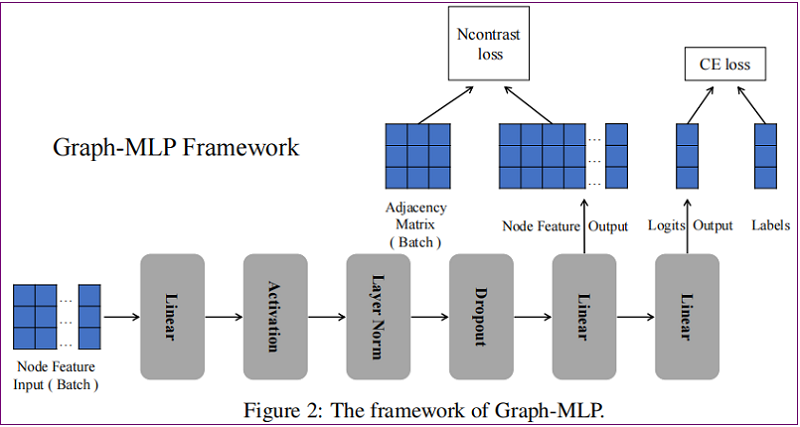
　　整体框架如下：

　　

class GMLP(nn.Module):
    def __init__(self, nfeat, nhid, nclass, dropout):
        super(GMLP, self).__init__()
        self.nhid = nhid
        self.mlp = Mlp(nfeat, self.nhid, dropout)
        self.classifier = Linear(self.nhid, nclass)

    def forward(self, x):
        Z = self.mlp(x)

        if self.training:
            x_dis = get_feature_dis(Z)

        class_feature = self.classifier(Z)
        class_logits = F.log_softmax(class_feature, dim=1)

        if self.training:
            return class_logits, x_dis
        else:
            return class_logits

2.1.1 MLP-based Structure

　　结构： linear-activation-layer normalization-dropout-linear-linear

　　即：

　　　　$\begin{array}{c} \mathbf{X}^{(1)}=\text { Dropout }\left(L N\left(\sigma\left(\mathbf{X} W^{0}\right)\right)\right) \quad\quad\quad(3)\\ \mathbf{Z}=\mathbf{X}^{(1)} W^{1} \quad\quad\quad(4)\\ \mathbf{Y}=\mathbf{Z} W^{2}\quad\quad\quad(5) \end{array}$

　　其中：$Z$ 用于 NConterast 损失，$ Y$ 用于分类损失。

2.1.2 Neighbouring Contrastive Loss

　　在 NContast 损失中，认为每个节点的 $\text{r-hop}$ 邻居为正样本，其他节点为负样本。这种损失鼓励正样本更接近目标节点，并根据特征距离推动负样本远离目标节点。采样 $B$ 个邻居，第 $i$ 个节点的 NContrast loss 可以表述为：

　　　　${\large \ell_{i}=-\log \frac{\sum\limits _{j=1}^{B} \mathbf{1}_{[j \neq i]} \gamma_{i j} \exp \left(\operatorname{sim}\left(\boldsymbol{z}_{i}, \boldsymbol{z}_{j}\right) / \tau\right)}{\sum\limits _{k=1}^{B} \mathbf{1}_{[k \neq i]} \exp \left(\operatorname{sim}\left(\boldsymbol{z}_{i}, \boldsymbol{z}_{k}\right) / \tau\right)}} \quad\quad\quad(6)$

　　其中：$\gamma_{i j} $ 表示节点 $i$ 和节点 $j$ 之间的连接强度，这里定义为 $\gamma_{i j}=\widehat{A}_{i j}^{r}$。

　　$\gamma_{i j}$ 为非 $0$ 值当且仅当结点 $j$ 是结点 $i$ 的 $r$  跳邻居，即： 

　　　　$\gamma_{i j}\left\{\begin{array}{ll}=0, & \text { node } j \text { is the } r \text {-hop neighbor of node } i \\\neq 0, & \text { node } j \text { is not the } r \text {-hop neighbor of node } i \end{array}\right.$

#计算特征相似度
def get_feature_dis(x):
    """
    x :           batch_size x nhid
    x_dis(i,j):   item means the similarity between x(i) and x(j).
    """
    x_dis = x@x.T

    x_sum = torch.sum(x**2, 1).reshape(-1, 1)
    x_sum = torch.sqrt(x_sum).reshape(-1, 1)
    x_sum = x_sum @ x_sum.T

    #标准化
    x_dis = x_dis*(x_sum**(-1))

    mask = torch.eye(x_dis.shape[0]).cuda(1)
    x_dis = (1-mask) * x_dis
    return x_dis

#定义 Ncontrast 损失函数
def Ncontrast(x_dis, adj_label, tau = 1):
    #分子计算
    x_dis = torch.exp( tau * x_dis)
    x_dis_sum_pos = torch.sum(x_dis * adj_label, 1)

    #分母计算
    x_dis_sum = torch.sum(x_dis, 1)

    #求平均
    # loss = -torch.log(x_dis_sum_pos * (x_dis_sum**(-1))+1e-8).mean()
    loss = -torch.log(x_dis_sum_pos * (x_dis_sum+1e-8) ** (-1)).mean()
    return loss

　　总 NContrast loss 为 $loss_{NC}$，而分类损失采用的是传统的交叉熵（用 $loss_{CE}$ 表示 )，因此上述 Graph-MLP 的总损失函数如下：

　　　　$\begin{aligned}\operatorname{loss}_{NC} &=\alpha \frac{1}{B} \sum\limits _{i=1}^{B} \ell_{i}\quad\quad\quad(7)\\\text { loss }_{\text {final }} &=\operatorname{loss}_{C E}+\operatorname{loss}_{N C}\quad\quad\quad(8) \end{aligned}$

def train():
    #获取Batch中的邻接矩阵和特征矩阵
    features_batch, adj_label_batch = get_batch(batch_size=args.batch_size)

    model.train()
    optimizer.zero_grad()
    output, x_dis = model(features_batch)

    loss_train_class = F.nll_loss(output[idx_train], labels[idx_train])  #分类损失

    loss_Ncontrast = Ncontrast(x_dis, adj_label_batch, tau = args.tau)  #邻居对比损失

    loss_train = loss_train_class + loss_Ncontrast * args.alpha
    acc_train = accuracy(output[idx_train], labels[idx_train])

    loss_train.backward()
    optimizer.step()
    return

2.1.3 Training

　　对用 Neighbouring Contrastive Loss 采用大小为 $B$ 的 batch 进行训练，对于分类损失按照本监督节点分类的设置进行计算。

　　算法如  Algorithm 1 所示：

　　

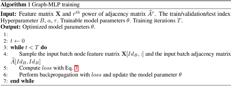
　　本文 Graph-MLP 输入的仅有属性信息，不依赖与结构信息，所以当结构信息发生变化时，Graph-MLP 仍然可以提供一致可靠的结果。

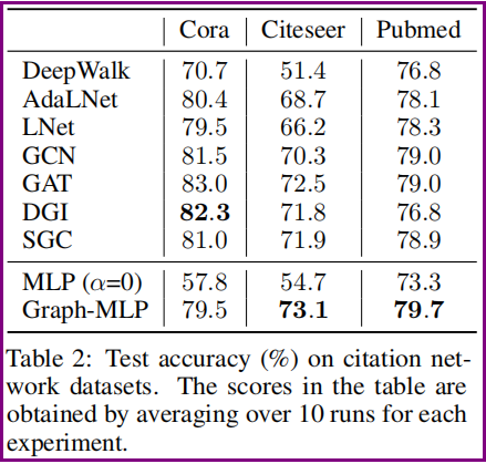
3 Experiment

数据集

　　

节点分类

　　

Graph-MLP 与 GNN 的效率对比

　　

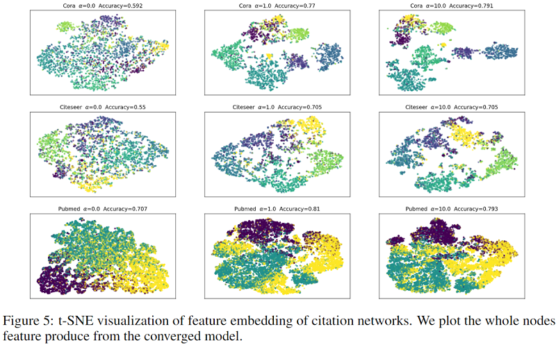
关于超参数的消融术研究

　　

可视化 

　　

鲁棒性

　　为了证明Graph-MLP在缺失连接下进行推断仍具有良好的鲁棒性，作者在测试过程中的邻接矩阵中添加了噪声，缺失连接的邻接矩阵的计算公式如下：

　　　　$A_{\text {corr }}=A \otimes  mask  +(1-  mask  ) \otimes \mathbb{N} \quad\quad\quad(9)$

　　　　$\operatorname{mask}\left\{\begin{array}{ll} =1, & p=1-\delta \\ =0, & p=\delta \end{array}\right.\quad\quad\quad(10)$

　　其中  $\delta$  表示缺失率，$mask  \in n \times n$  决定邻接矩阵中缺失的位置，$mask$ 中的元素取  $1 / 0$  的概率为  $1-\delta / \delta$ 。 $\mathbb{N} \in n \times n$  中的元素取  $1 / 0$  的 概率都为  $0.5$  。

　　

　　结论：从上图可以看出随着缺失率的增加，GCN的推断性能急剧下降，而Graph-MLP却基本不受影响。

4 Conclusion

　　提出邻居对比损失，输入仅依赖于属性信息，并不依赖结构信息。

 

修改历史

2022-04-02 创建文章
2022-06-12 精读

 

论文解读目录