深度学习基础理论————混合专家模型(MoE)/KV-cache
1、混合专家模型(MoE)
参考HuggingFace中介绍:混合专家模型主要由两部分构成:
1、稀疏的MoE层:这些层代替了传统 Transformer 模型中的前馈网络 (FFN) 层。MoE 层包含若干“专家”(例如 8 个),每个专家本身是一个独立的神经网络。在实际应用中,这些专家通常是前馈网络 (FFN),但它们也可以是更复杂的网络结构,甚至可以是 MoE 层本身,从而形成层级式的 MoE 结构。
2、门控网络/路由(Gate Layer/route Layer):这个部分用于决定哪些令牌 (token) 被发送到哪个专家。例如,在下图中,“More”这个令牌可能被发送到第二个专家,而“Parameters”这个令牌被发送到第一个专家。有时,一个令牌甚至可以被发送到多个专家。令牌的路由方式是 MoE 使用中的一个关键点,因为路由器由学习的参数组成,并且与网络的其他部分一同进行预训练。
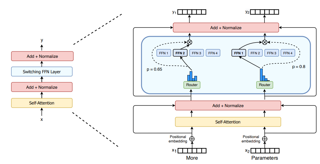
换言之也就是说:将原始的Transformer框架中的FFN Layer(全连接层)替换成一个由Gate Layer和若干的FFN Layer组成的结构,通过Gate来确定一个输入将会被那些FFN进行处理,而后对被FFN处理后的内容进行加权处理。
- 1、稠密MoE和 稀疏MoE
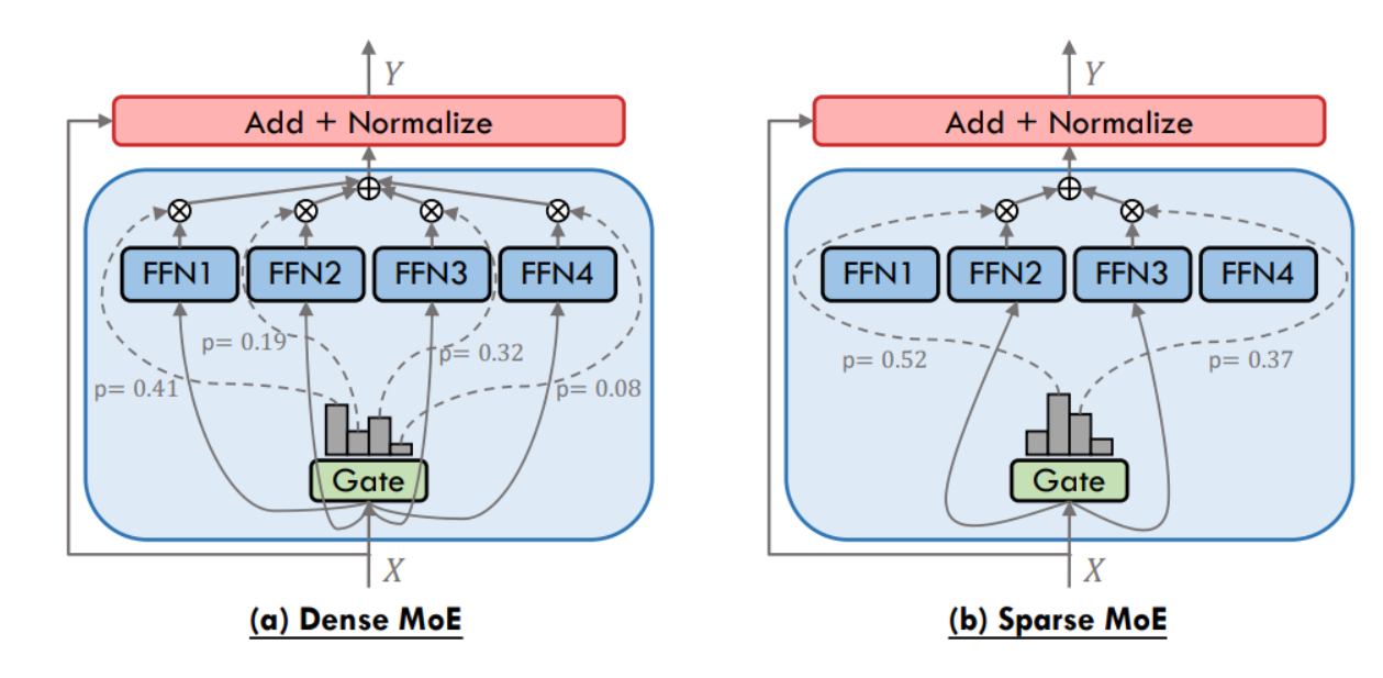
检验而言:如上图所示,对于稠密的MoE(Dense MoE)而言(假设4个FFN)在通过Gate处理之后输入X要通过每一个FFN进行处理,而对于稀疏的MoE(Sparse MoE)而言,通过Gate处理只去选择部分FFN进行处理
- 2、
MoE原理
1、Gate/route原理
输入数据\(x\),通过一个线性层进行处理:
对于得到的score再通过Softmax函数处理,得到一个概率分布:
对于稀疏的MoE而言还需要去选择部分专家进行激活:
原理很简单,结合代码分析(以Deepseek-v3代码为例)
class Gate(nn.Module):
    """
    Gating mechanism for routing inputs in a mixture-of-experts (MoE) model.
    """
    def __init__(self, args: ModelArgs):
        """
        Initializes the Gate module.

        Args:
            args (ModelArgs): Model arguments containing gating parameters.
        """
        super().__init__()
        self.dim = args.dim
        self.topk = args.n_activated_experts # 选择多少个专家进行使用
        self.n_groups = args.n_expert_groups # Gate数量
        self.topk_groups = args.n_limited_groups # 对于gate中分组数
        self.score_func = args.score_func
        self.route_scale = args.route_scale
        self.weight = nn.Parameter(torch.empty(args.n_routed_experts, args.dim))
        self.bias = nn.Parameter(torch.empty(args.n_routed_experts)) if self.dim == 7168 else None

    def forward(self, x: torch.Tensor) -> Tuple[torch.Tensor, torch.Tensor]:
        """
        Forward pass for the gating mechanism.

        Args:
            x (torch.Tensor): Input tensor.

        Returns:
            Tuple[torch.Tensor, torch.Tensor]: Routing weights and selected expert indices.
        """
        scores = linear(x, self.weight) # 计算wx+b
        # 归一化处理
        if self.score_func == "softmax":
            scores = scores.softmax(dim=-1, dtype=torch.float32)
        else:
            scores = scores.sigmoid()
        original_scores = scores

        if self.bias is not None:
            scores = scores + self.bias
        if self.n_groups > 1:
            # 如果Gate数量>1
            scores = scores.view(x.size(0), self.n_groups, -1)
            if self.bias is None:
                group_scores = scores.amax(dim=-1)
            else:
                group_scores = scores.topk(2, dim=-1)[0].sum(dim=-1)
            indices = group_scores.topk(self.topk_groups, dim=-1)[1]
            mask = torch.zeros_like(scores[..., 0]).scatter_(1, indices, True)
            scores = (scores * mask.unsqueeze(-1)).flatten(1)
        indices = torch.topk(scores, self.topk, dim=-1)[1]
        weights = original_scores.gather(1, indices)
        if self.score_func == "sigmoid":
            weights /= weights.sum(dim=-1, keepdim=True)
        weights *= self.route_scale
        return weights.type_as(x), indices
整个过程分析:输入数据x(假设维度为:(bs, num_tokens, embed_dim)),通过线性(W:(n_routed_experts,embed_dim)计算得到:bs,num_tokens,n_routed_experts)和归一化处理:(bs,num_tokens, n_routed_experts)这样一来就可以知道每个tokens的一个分布概率(到底要走哪一个FFN)。如果n_expert_groups数量>1,也就是说如果Gate数量不止一个,那么也就只需要去选择topK即可然后用一个mask将其他的给mask掉即可(scores = (scores * mask.unsqueeze(-1)).flatten(1))然后再去对挑选得到的Gate选择topk(indices = torch.topk(scores, self.topk, dim=-1)[1])
2、FFN Layer原理
这部分代码就比较简单(直接用线性层处理即可):
class Expert(nn.Module):
    """
    Expert layer for Mixture-of-Experts (MoE) models.

    Attributes:
        w1 (nn.Module): Linear layer for input-to-hidden transformation.
        w2 (nn.Module): Linear layer for hidden-to-output transformation.
        w3 (nn.Module): Additional linear layer for feature transformation.
    """
    def __init__(self, dim: int, inter_dim: int):
        """
        Initializes the Expert layer.

        Args:
            dim (int): Input and output dimensionality.
            inter_dim (int): Hidden layer dimensionality.
        """
        super().__init__()
        self.w1 = Linear(dim, inter_dim)
        self.w2 = Linear(inter_dim, dim)
        self.w3 = Linear(dim, inter_dim)

    def forward(self, x: torch.Tensor) -> torch.Tensor:
        """
        Forward pass for the Expert layer.

        Args:
            x (torch.Tensor): Input tensor.

        Returns:
            torch.Tensor: Output tensor after expert computation.
        """
        return self.w2(F.silu(self.w1(x)) * self.w3(x))
最后得到MoE代码如下:
class MoE(nn.Module):
    """
    Mixture-of-Experts (MoE) module.

    Attributes:
        dim (int): Dimensionality of input features.
        n_routed_experts (int): 模型中总的专家数量
        n_local_experts (int): 在分布式系统中,当前设备(节点)负责的专家数量
        n_activated_experts (int): 每个输入激活的专家数量(即每个输入会被路由到多少个专家)。
        gate (nn.Module): Gating mechanism to route inputs to experts.
        experts (nn.ModuleList): List of expert modules.
        shared_experts (nn.Module): Shared experts applied to all inputs.
    """
    def __init__(self, args: ModelArgs):
        """
        Initializes the MoE module.

        Args:
            args (ModelArgs): Model arguments containing MoE parameters.
        """
        super().__init__()
        self.dim = args.dim
        assert args.n_routed_experts % world_size == 0
        self.n_routed_experts = args.n_routed_experts
        self.n_local_experts = args.n_routed_experts // world_size
        self.n_activated_experts = args.n_activated_experts

        # 起始/结束(因为是涉及到分布训练,去寻找每个设备上的”专家“即可)
        self.experts_start_idx = rank * self.n_local_experts
        self.experts_end_idx = self.experts_start_idx + self.n_local_experts

        self.gate = Gate(args)
        self.experts = nn.ModuleList([Expert(args.dim, args.moe_inter_dim) if self.experts_start_idx <= i < self.experts_end_idx else None
                                      for i in range(self.n_routed_experts)])
        self.shared_experts = MLP(args.dim, args.n_shared_experts * args.moe_inter_dim)

    def forward(self, x: torch.Tensor) -> torch.Tensor:
        """
        Forward pass for the MoE module.

        Args:
            x (torch.Tensor): Input tensor.

        Returns:
            torch.Tensor: Output tensor after expert routing and computation.
        """
        shape = x.size()
        x = x.view(-1, self.dim)
        weights, indices = self.gate(x)
        y = torch.zeros_like(x)
        counts = torch.bincount(indices.flatten(), minlength=self.n_routed_experts).tolist()
        for i in range(self.experts_start_idx, self.experts_end_idx):
            if counts[i] == 0:
                continue
            expert = self.experts[i]
            idx, top = torch.where(indices == i)
            y[idx] += expert(x[idx]) * weights[idx, top, None]
        z = self.shared_experts(x)
        if world_size > 1:
            dist.all_reduce(y)
        return (y + z).view(shape)
代码分析:
1、获取权重以及索引:weights, indices = self.gate(x)
2、计算每个专家索引:counts = torch.bincount(indices.flatten(), minlength=self.n_routed_experts).tolist()通过torch.bincount返回数值个数,比如说:[1,2,2,2,3],那么返回:[0,1,3,1](0出现0次,1出现1次。。。。)相当于对每个专家都编号了,只需要根据出现次数,来索引出来
3、计算加权得分:
for i in range(self.experts_start_idx, self.experts_end_idx):
    if counts[i] == 0:
        continue
    expert = self.experts[i]
    idx, top = torch.where(indices == i)
    y[idx] += expert(x[idx]) * weights[idx, top, None]
如果涉及到多个专家,很可能就会出现一种情况:只有部分的专家被使用进而导致负载不均衡。那么可以通过 负载均衡损失(Load Balancing Loss)(如上图所示)计算主要为:
1、importance loss(重要性损失)
回到上面对于router函数(\(s = \text{softmax}(W_{gate}x+b)\))在论文中对于重要性损失定义如下:
也就是说,通过最小化上式子的最小值(均值大,方差小),进而保证所有的专家平均而言拥有相似的权重。
2、Load Loss:重要性损失旨在保证所有专家平均而言具有相似的路由权重。但是不难想到这些看上去有着总体趋于平衡的权重的路由配置,仍然有一小部分专家获得了所有分配,如下图:

首先,对于专家选择阈值:\(threshold_k(x):= max_k(Wx+ \phi)\),其中\(\phi\)代表前向传播过程中的采样噪声,\(max_k\)代表选择第\(k\)个最大的值,对于专家的负载:指的是在整个批次中的使用情况:\(load_i(X)=\sum_{x\in X}p_i(x)\)对于这个概率的计算:
其中\(\phi_{\mathrm{new}}\sim\mathcal{N}(0,\sigma^{2}),\sigma=1/E\)最后对于load loss定义为:
最后损失函数为:\(L=\frac{1}{2}L_{importance}(X)+ \frac{1}{2}L_{load}(X)\)
同时也可以采用另外的方法:
1、GShard设定一个 专家容量:设定一个阈值,定义一个专家能处理多少令牌。如果两个专家的容量都达到上限,令牌就会溢出,并通过残差连接传递到下一层,或在某些情况下被完全丢弃。对于专家容量可以借鉴下面处理方式:\(\frac{\text{tokens per batch}}{\text{number of experts}}\times \text{capacity factor}\)(\(\text{capacity factor}\)可以选择1-1.25之间)
KV cache
Transformer模型推理过程为:
目前主流的LLM框架主要都是使用的decoder-only(也就是说只用Transformer中的decoder结构)
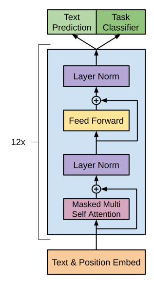
对于LLM任务(通常采用自回归过程)可以简单认为是一种“完形填空”的过程,在输入前面i-1个词然后推测第i个词
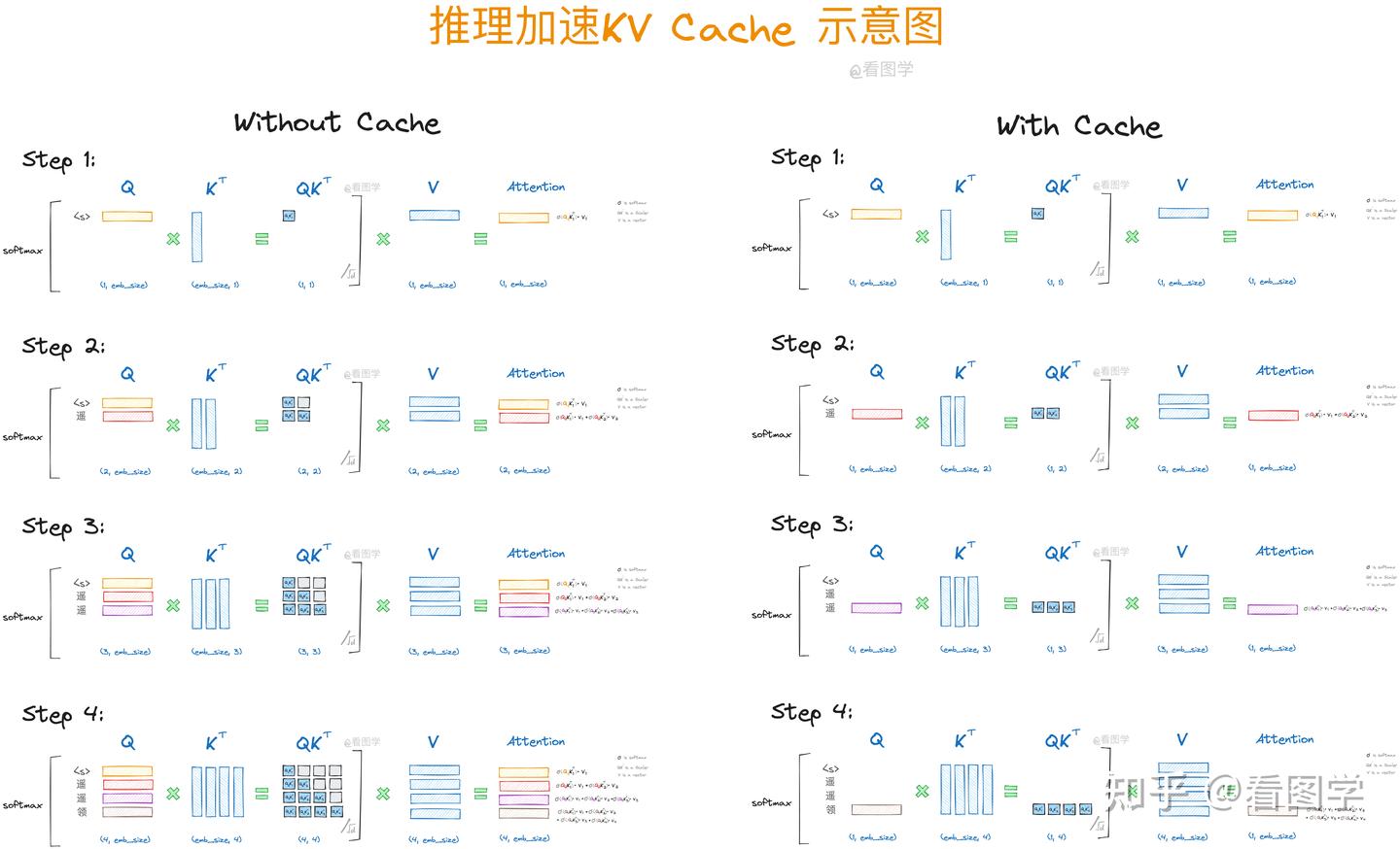
回归上面的推理过程(翻译输出:i am a student):模型中在输出'a'的时候会将'i am'都输入到模型中。理解这个过程(假设就是直接输出文本:i am a student):
step1: in: Q=K<S> || out: i
\(Attention_1: Q_1K_1^T\)
step2: in: Q=K=<s>,i || out: i am
\(Attention_1: Q_1K_1^T \\ Attention_2:Q_2K_1^T, Q_2K_2^T\)
step3: in: Q=K=<s>, i, am || out: i am a
\(Attention_1: Q_1K_1^T \\ Attention_2:Q_2K_1^T, Q_2K_2^T \\
Attention_3: Q_3K_1^T, Q_3K_2^T, Q_3K_3^T\)
step4: in: Q=K=<s>, i, am, a || out: i am a student
\(Attention_1: Q_1K_1^T \\ Attention_2:Q_2K_1^T, Q_2K_2^T \\
Attention_3: Q_3K_1^T, Q_3K_2^T, Q_3K_3^T \\
Attention_4: Q_4K_1^T, Q_4K_2^T, Q_4K_3^T, Q_4K_4^T
\)
不过上面操作过程中会有问题:
计算有很大冗余(每次生成新的词,都需要回归一下之前生成的词),并且每次计算\(Attention_i\)只与\(Q_i\)相关
对于后面一点理解(以step2为例):
我目前已经有两个\(Q\):\(Q_1:<s>\, Q_2:\text{i}\) 并且还有K和V(这两个也是有两个值),我会初始化一个\(Q_3\)对于下一个值我就用\(Q_3\)进行表示,然后我就需要去计算注意力得分(只用Q,K,V这三个值计算过程举例):
\(QK^T=(bs, 3, embed_{dim})(bs, embed_dim, 2)=(bs, 3, 2)\),接下来计算\(QK^TV=(bs, 3, 2)(bs,2,embed_dim)=(bs, 3, embed_dim)\)那么在这个过程中就会有一个有意思问题:Q会有重复的(dim=3,前面两个都是前面已经计算过的)(观察上面Attention计算可以发现:每次计算\(Attention_i\)只与\(Q_i\)相关)。因此就有KV-cache理论:既然每次都是Q在变化,但是K和V都是用的之前的,那我之前每次就只用新的Q去和旧的KV计算即可(将KV存储起来),KV-cache一种典型的用内存换速度的方法
简易Demo:
import torch

class KVCache:
    def __init__(self):
        self.k = None
        self.v = None

    def update(self, k, v):
        if self.k is None:
            self.k = k
            self.v = v
        else:
            self.k = torch.cat([self.k, k], dim=1)  # 在序列维度上拼接
            self.v = torch.cat([self.v, v], dim=1)

    def get(self):
        return self.k, self.v

class Decoder(torch.nn.Module):
    def __init__(self, embed_dim, hidden_dim, vocab_size, num_heads=8):
        super().__init__()
        self.embedding = torch.nn.Embedding(vocab_size, embed_dim)
        self.attention = torch.nn.MultiheadAttention(embed_dim, num_heads)
        self.linear = torch.nn.Linear(embed_dim, vocab_size)
        self.kv_cache = KVCache()

    def forward(self, input_ids):
        x = self.embedding(input_ids)  # (batch_size, seq_len, embed_dim)

        # 获取 KV-cache
        k, v = self.kv_cache.get()

        # 计算 Attention
        if k is not None and v is not None:
            # 使用 KV-cache
            attn_output, _ = self.attention(x, k, v)  # (batch_size, seq_len, embed_dim)
        else:
            # 初始状态,没有 KV-cache
            attn_output, _ = self.attention(x, x, x)  # (batch_size, seq_len, embed_dim)

        # 更新 KV-cache
        self.kv_cache.update(x, x)

        # 残差连接
        x = x + attn_output

        # 线性变换
        logits = self.linear(x)  # (batch_size, seq_len, vocab_size)

        return logits

batch_size = 2
seq_len = 4
embed_dim = 64
hidden_dim = 256
vocab_size = 10000  # 假设词汇表大小为 10000
decoder = Decoder(embed_dim, hidden_dim, vocab_size)
input_ids = torch.randint(0, vocab_size, (batch_size, seq_len))  # (batch_size, seq_len)
logits = decoder(input_ids)  # (batch_size, seq_len, vocab_size)
print("Logits shape:", logits.shape)
使用Huggingface的transformers框架代码: https://huggingface.co/docs/transformers/main/en/kv_cache 。只需要类似下面操作:
import torch
from transformers import AutoTokenizer, AutoModelForCausalLM
ckpt = "microsoft/Phi-3-mini-4k-instruct"

tokenizer = AutoTokenizer.from_pretrained(ckpt)
model = AutoModelForCausalLM.from_pretrained(ckpt, torch_dtype=torch.float16).to("cuda:0")
inputs = tokenizer("Fun fact: The shortest", return_tensors="pt").to(model.device)

# 具体参数:https://huggingface.co/docs/transformers/en/main_classes/text_generation
out = model.generate(**inputs, do_sample=False, max_new_tokens=23, use_cache=True)
print(tokenizer.batch_decode(out, skip_special_tokens=True)[0])

out = model.generate(**inputs, do_sample=False, max_new_tokens=23)
print(tokenizer.batch_decode(out, skip_special_tokens=True)[0])
在Transformers中不同cache方式:
| 缓存类型 | 描述 | 适用场景 | 优点 | 缺点 |
|---|---|---|---|---|
| StaticCache | 静态缓存,缓存所有的 K 和 V,不更新。 | 短序列生成、内存充足的场景 | 实现简单,快速 | 不适合长序列生成,内存消耗较大 |
| OffloadedStaticCache | 静态缓存,但将缓存内容卸载到外部存储。 | 内存受限的环境,长序列生成 | 减少显存占用,适合大规模生成 | 存取速度较慢,可能影响生成速度 |
| SlidingWindowCache | 滑动窗口缓存,缓存一个固定大小的窗口。 | 长序列生成、内存有限的场景 | 限制内存消耗,适合长序列生成 | 窗口太小可能丢失上下文信息,影响生成效果 |
| HybridCache | 混合缓存,结合静态缓存和滑动窗口缓存。 | 长序列生成,要求平衡内存和上下文 | 平衡内存消耗和上下文保留 | 比静态缓存更复杂,可能需要更多内存管理和计算资源 |
| MambaCache | 高效的缓存实现,针对推理速度和内存占用进行了优化。 | 高性能计算环境、高并发推理任务 | 高度优化,适合大规模并行推理 | 可能需要特定硬件支持,复杂度较高 |
| QuantizedCache | 量化缓存,减少存储需求。 | 内存受限的设备、需要减少内存占用的场景 | 大幅度减少内存占用,适合嵌入式设备 | 量化可能导致精度损失,影响生成质量 |
争对上面描述其实KV-cahce是一种用存储换速度的方法,因此,对于KV存储进行优化就十分有必要了!
参考
1、https://arxiv.org/pdf/2101.03961
2、混合专家模型 (MoE) 详解
3、https://arxiv.org/pdf/2407.06204
4、https://github.com/deepseek-ai/DeepSeek-V3/blob/main/inference/model.py
5、https://arxiv.org/pdf/2106.05974
6、https://arxiv.org/pdf/2006.16668
7、https://cdn.openai.com/research-covers/language-unsupervised/language_understanding_paper.pdf
8、https://jalammar.github.io/illustrated-transformer/
9、https://zhuanlan.zhihu.com/p/662498827

 浙公网安备 33010602011771号