KNN(一)

目录

• 基础知识梳理：
• 实现

基础知识梳理：

实现

import matplotlib.pyplot as plt
import numpy as np
import operator

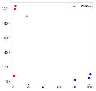
#已知分类的数据
x_data=np.array([[3,104],
                 [2,100],
                 [1,8],
                 [101,10],
                 [99,5],
                 [81,2]])
y_data=np.array(["A",'A',"A","B","B","B"])
x_test=np.array([18,90])

#plt.scatter(x_data[:,0],x_data[:,1],c=y_data)
#颜色
col_dict={i:j for i,j in zip(set(y_data),['b','r'])}
plt.figure(figsize=(5,5))
for x,y,c in zip(x_data[:,0],x_data[:,1],y_data):
    plt.scatter(x,y,c=col_dict[c])
plt.scatter(x_test[0],x_test[1],marker='*',label='unknow')
plt.legend()
plt.show()

#计算样本数量
x_data.shape

(6, 2)

def knn(x_test,x_data,y_data,k):
    """
    @params:x_test未知样本
    @params:x_data 带标签样本
    @params:k：类的个数
    """
    #计算样本距离
    dis=((x_data-x_test)**2).sum(axis=1)**0.5
    #距离从小到大排序，获取对应样例所在的位置
    sortedDis=dis.argsort()
    #统计最近邻的K个样例中每一个标签出现的次数
    classCount={}
    for i in range(k):
        voteLabel=y_data[sortedDis[i]]
        classCount[voteLabel]=classCount.get(voteLabel,0)+1
    #对统计结果(字典)排序
    sortedClassCount=sorted(classCount.items(),key=lambda x:x[1],reverse=True)
    print('当前样本的预测标签：%s'%sortedClassCount[0][0],"对应的概率:%s"%dict([(i[0],i[1]/k)for i in sortedClassCount]))
    return sortedClassCount[0][0]

#运行结果
knn(x_test,x_data,y_data,5)

当前样本的预测标签：A 对应的概率:{'A': 0.6, 'B': 0.4}





'A'

#调包
from sklearn import neighbors

k_neigh=5
neigh=neighbors.KNeighborsClassifier(k_neigh,weights='distance')
neigh.fit(x_data,y_data)

KNeighborsClassifier(algorithm='auto', leaf_size=30, metric='minkowski',
                     metric_params=None, n_jobs=None, n_neighbors=5, p=2,
                     weights='distance')

print("预测标签%s"%neigh.predict([x_test]))
print('预测概率%s'%neigh.predict_proba([x_test]))

预测标签['A']
预测概率[[0.86386355 0.13613645]]

import numpy as np
from sklearn import datasets
from sklearn.model_selection import train_test_split
from sklearn.metrics import classification_report,confusion_matrix
import random

#载入数据
#### Iris数据集
iris=datasets.load_iris()
#划分数据集
x_train,x_test,y_train,y_test=train_test_split(iris.data,iris.target,test_size=0.2)

# #打乱数据
# data_size=iris.data.shape[0]
# index=[i for i in range(data_size)]
# random.shuffle(index)
# iris.data=iris.data[index]
# iris.target=iris.target[index]
# #切分数据集
# test_size=40
# x_train=iris.data[test_size:]
# x_test=iris.data[:test_size]
# y_train=iris.target[test_size:]
# y_test=iris.target[:test_size]

predictions=[]
for i in range(x_test.shape[0]):
    predictions.append(knn(x_test[i],x_train,y_train,10))
print(classification_report(y_test,predictions))

当前样本的预测标签：0 对应的概率:{0: 1.0}
当前样本的预测标签：1 对应的概率:{1: 1.0}
当前样本的预测标签：2 对应的概率:{2: 1.0}
当前样本的预测标签：2 对应的概率:{2: 1.0}
当前样本的预测标签：0 对应的概率:{0: 1.0}
当前样本的预测标签：1 对应的概率:{1: 1.0}
当前样本的预测标签：2 对应的概率:{2: 1.0}
当前样本的预测标签：1 对应的概率:{1: 1.0}
当前样本的预测标签：1 对应的概率:{1: 0.8, 2: 0.2}
当前样本的预测标签：1 对应的概率:{1: 1.0}
当前样本的预测标签：2 对应的概率:{2: 0.6, 1: 0.4}
当前样本的预测标签：2 对应的概率:{2: 0.8, 1: 0.2}
当前样本的预测标签：1 对应的概率:{1: 0.6, 2: 0.4}
当前样本的预测标签：1 对应的概率:{1: 1.0}
当前样本的预测标签：1 对应的概率:{1: 1.0}
当前样本的预测标签：2 对应的概率:{2: 1.0}
当前样本的预测标签：2 对应的概率:{2: 0.6, 1: 0.4}
当前样本的预测标签：2 对应的概率:{2: 1.0}
当前样本的预测标签：2 对应的概率:{2: 1.0}
当前样本的预测标签：0 对应的概率:{0: 1.0}
当前样本的预测标签：1 对应的概率:{1: 1.0}
当前样本的预测标签：1 对应的概率:{1: 0.9, 2: 0.1}
当前样本的预测标签：1 对应的概率:{1: 0.7, 2: 0.3}
当前样本的预测标签：1 对应的概率:{1: 0.8, 2: 0.2}
当前样本的预测标签：0 对应的概率:{0: 1.0}
当前样本的预测标签：2 对应的概率:{2: 1.0}
当前样本的预测标签：0 对应的概率:{0: 1.0}
当前样本的预测标签：1 对应的概率:{1: 1.0}
当前样本的预测标签：0 对应的概率:{0: 1.0}
当前样本的预测标签：2 对应的概率:{2: 1.0}
              precision    recall  f1-score   support

           0       1.00      1.00      1.00         6
           1       0.92      0.86      0.89        14
           2       0.82      0.90      0.86        10

    accuracy                           0.90        30
   macro avg       0.91      0.92      0.92        30
weighted avg       0.90      0.90      0.90        30

confusion_matrix(y_test,predictions)

array([[ 6,  0,  0],
       [ 0, 12,  2],
       [ 0,  1,  9]], dtype=int64)

---

import numpy as np
import matplotlib.pyplot as plt
from matplotlib.colors import ListedColormap
from sklearn import neighbors, datasets

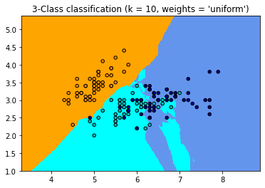
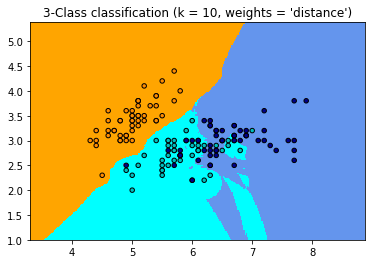
n_neighbors = 10

# import some data to play with
iris = datasets.load_iris()

# we only take the first two features. We could avoid this ugly
# slicing by using a two-dim dataset
X = iris.data[:, :2]
y = iris.target

h = .02  # step size in the mesh

# Create color maps
cmap_light = ListedColormap(['orange', 'cyan', 'cornflowerblue'])
cmap_bold = ListedColormap(['darkorange', 'c', 'darkblue'])

for weights in ['uniform', 'distance']:
    # we create an instance of Neighbours Classifier and fit the data.
    clf = neighbors.KNeighborsClassifier(n_neighbors, weights=weights)
    clf.fit(X, y)

    # Plot the decision boundary. For that, we will assign a color to each
    # point in the mesh [x_min, x_max]x[y_min, y_max].
    x_min, x_max = X[:, 0].min() - 1, X[:, 0].max() + 1
    y_min, y_max = X[:, 1].min() - 1, X[:, 1].max() + 1
    xx, yy = np.meshgrid(np.arange(x_min, x_max, h),
                         np.arange(y_min, y_max, h))
    Z = clf.predict(np.c_[xx.ravel(), yy.ravel()])

    # Put the result into a color plot
    Z = Z.reshape(xx.shape)
    plt.figure()
    plt.pcolormesh(xx, yy, Z, cmap=cmap_light)

    # Plot also the training points
    plt.scatter(X[:, 0], X[:, 1], c=y, cmap=cmap_bold,
                edgecolor='k', s=20)
    plt.xlim(xx.min(), xx.max())
    plt.ylim(yy.min(), yy.max())
    plt.title("3-Class classification (k = %i, weights = '%s')"
              % (n_neighbors, weights))

plt.show()

Automatically created module for IPython interactive environment

-->>>关于sklearn中关于KNN的实现，将单独整理成篇！

---

参考:
《机器学习实战》
sklearn中KNN的实现