Tensorflow（一） TensorFlow基础

开始学习TensorFlow：https://www.tensorflow.org/tutorials

TensorFlow的官网上有Tutorial和Guide两部分教程，Guide主要介绍一些概念性的东西，Tutorial则更加通过实例来介绍TensorFlow的使用。

本篇介绍TensorFlow基础，参考：https://www.tensorflow.org/guide/basics

TensorFlow 基础

TensorFlow是一个端到端的机器学习平台。支持以下功能:

• 基于多维数组的数值计算(类似于NumPy)。
• GPU与分布式处理
• 自动分化
• 模型构建、训练、输出

Tensors

Tensor是TensorFlow中的基本数据存储单元，下为一个二维的tensor：

import tensorflow as tf

x = tf.constant([[1., 2., 3.],
                 [4., 5., 6.]])

print(x)
print(x.shape)
print(x.dtype)

tf.Tensor(
[[1. 2. 3.]
[4. 5. 6.]], shape=(2, 3), dtype=float32)
(2, 3)
<dtype: 'float32'>

类似Numpy， tf.Tensor 中的shape和dtype属性:

• Tensor.shape: tells you the size of the tensor along each of its axes.
• Tensor.dtype: tells you the type of all the elements in the tensor.

TensorFlow实现了对tensor的标准数学运算，以及许多专门用于机器学习的运算。

如：

x + x

<tf.Tensor: shape=(2, 3), dtype=float32, numpy=
array([[ 2., 4., 6.],
[ 8., 10., 12.]], dtype=float32)>

5 * x

<tf.Tensor: shape=(2, 3), dtype=float32, numpy=
array([[ 5., 10., 15.],
[20., 25., 30.]], dtype=float32)>

x @ tf.transpose(x)

<tf.Tensor: shape=(2, 2), dtype=float32, numpy=
array([[14., 32.],
[32., 77.]], dtype=float32)>

tf.concat([x, x, x], axis=0)

<tf.Tensor: shape=(6, 3), dtype=float32, numpy=
array([[1., 2., 3.],
[4., 5., 6.],
[1., 2., 3.],
[4., 5., 6.],
[1., 2., 3.],
[4., 5., 6.]], dtype=float32)>

tf.nn.softmax(x, axis=-1)

<tf.Tensor: shape=(2, 3), dtype=float32, numpy=
array([[0.09003057, 0.24472848, 0.66524094],
[0.09003057, 0.24472848, 0.66524094]], dtype=float32)>

tf.reduce_sum(x)

<tf.Tensor: shape=(), dtype=float32, numpy=21.0>

在CPU上运行大型计算可能很慢。当正确配置时，TensorFlow可以使用gpu等加速硬件来快速执行操作。

if tf.config.list_physical_devices('GPU'):
  print("TensorFlow **IS** using the GPU")
else:
  print("TensorFlow **IS NOT** using the GPU")

TensorFlow IS NOT using the GPU

Variables

通常 tf.Tensor 是不可变的， 在TensorFlow中存储如权重这样的变量用tf.Variable.

var = tf.Variable([0.0, 0.0, 0.0])

var.assign([1, 2, 3])

<tf.Variable 'UnreadVariable' shape=(3,) dtype=float32, numpy=array([1., 2., 3.], dtype=float32)>

var.assign_add([1, 1, 1])

<tf.Variable 'UnreadVariable' shape=(3,) dtype=float32, numpy=array([2., 3., 4.], dtype=float32)>

Gradient Descent

Gradient descent 自动分化是机器学习算法的基础

为了实现这一点，TensorFlow实现了自动微分(autodiff)，它使用微积分来计算梯度。通常，您将使用它来计算模型的_error_或_loss相对于其权重的梯度。

x = tf.Variable(1.0)

def f(x):
  y = x**2 + 2*x - 5
  return y

f(x)

<tf.Tensor: shape=(), dtype=float32, numpy=-2.0>

在x = 1.0处，y = f(x) = (1**2 + 2*1 - 5) = -2

y的导数是y = f'(x) = (2*x + 2) = 4 TensorFlow可以自动计算:

with tf.GradientTape() as tape:
  y = f(x)

g_x = tape.gradient(y, x)  # g(x) = dy/dx

g_x

<tf.Tensor: shape=(), dtype=float32, numpy=4.0>

这个简化的例子只对单个标量(' x ')求导，但TensorFlow可以同时计算对任意数量的非标量Tensor的梯度。

Graphs & tf.function

TensorFlow提供了以下功能:

• Performance optimization: 加速训练和推理.
• Export: 导出训练好的模型.

这需要 tf.function 相关功能支持

@tf.function
def my_func(x):
  print('Tracing.\n')
  return tf.reduce_sum(x)

参考： https://www.tensorflow.org/guide/function
通过tf.functionDecorator，对函数进行Tensor加速的操作

x = tf.constant([1, 2, 3])
my_func(x)

Tracing.
<tf.Tensor: shape=(), dtype=int32, numpy=6>

在随后的调用中，TensorFlow只执行优化后的图，跳过任何非TensorFlow步骤。注意'my_func 不会打印_tracing_，因为print 是一个Python函数，而不是TensorFlow函数。

x = tf.constant([10, 9, 8])
my_func(x)

<tf.Tensor: shape=(), dtype=int32, numpy=27>

一个graph不会随着不同_signature_ (shape and dtype)的输入而重用，定义一个新的graph:

x = tf.constant([10.0, 9.1, 8.2], dtype=tf.float32)
my_func(x)

Tracing.
<tf.Tensor: shape=(), dtype=float32, numpy=27.3>

这些Graph提供了两个好处:

• 在许多情况下，它们提供了显著的执行速度。
• 您可以使用tf导出这些图形。saved_model，在服务器或移动设备等其他系统上运行，不需要安装Python。

Modules, layers, models

tf.Module 是一个用来管理 tf.Variable 对象的类，tf.function提供方法用来操作它们。
tf.Module 包含了2个显著的特征：

1. 你可以使用tf.train.Checkpoint来保存和恢复变量的值。这在训练期间很有用，因为它可以快速保存和恢复模型的状态。
2. 您可以导入和导出tf.variable变量的值, tf.function使用tf.saved_model的函数图。这允许您独立于创建模型的Python程序运行模型。

tf.Module完整示例：

class MyModule(tf.Module):
  def __init__(self, value):
    self.weight = tf.Variable(value)

  @tf.function
  def multiply(self, x):
    return x * self.weight

mod = MyModule(3)
mod.multiply(tf.constant([1, 2, 3]))

<tf.Tensor: shape=(3,), dtype=int32, numpy=array([3, 6, 9], dtype=int32)>

存储 Module:

save_path = './saved'
tf.saved_model.save(mod, save_path)

INFO:tensorflow:Assets written to: ./saved/assets
2022-01-19 02:29:48.135588: W tensorflow/python/util/util.cc:368] Sets are not currently considered sequences, but this may change in the future, so consider avoiding using them.

SavedModel的存出结果与代码相互独立，你可以通过Python载入它，或者是其它语言。也可以用于TensorFlow Serving，或者用于TensorFlow Lite 或TensorFlow JS.

reloaded = tf.saved_model.load(save_path)
reloaded.multiply(tf.constant([1, 2, 3]))

<tf.Tensor: shape=(3,), dtype=int32, numpy=array([3, 6, 9], dtype=int32)>

tf.keras.layers.Layer 和 tf.keras.Model 基于Module构建，为构建、训练和保存模型提供额外的功能和方便的方法。

Training loops

现在把这些都放在一起，建立一个基本的模型，从头开始训练它。

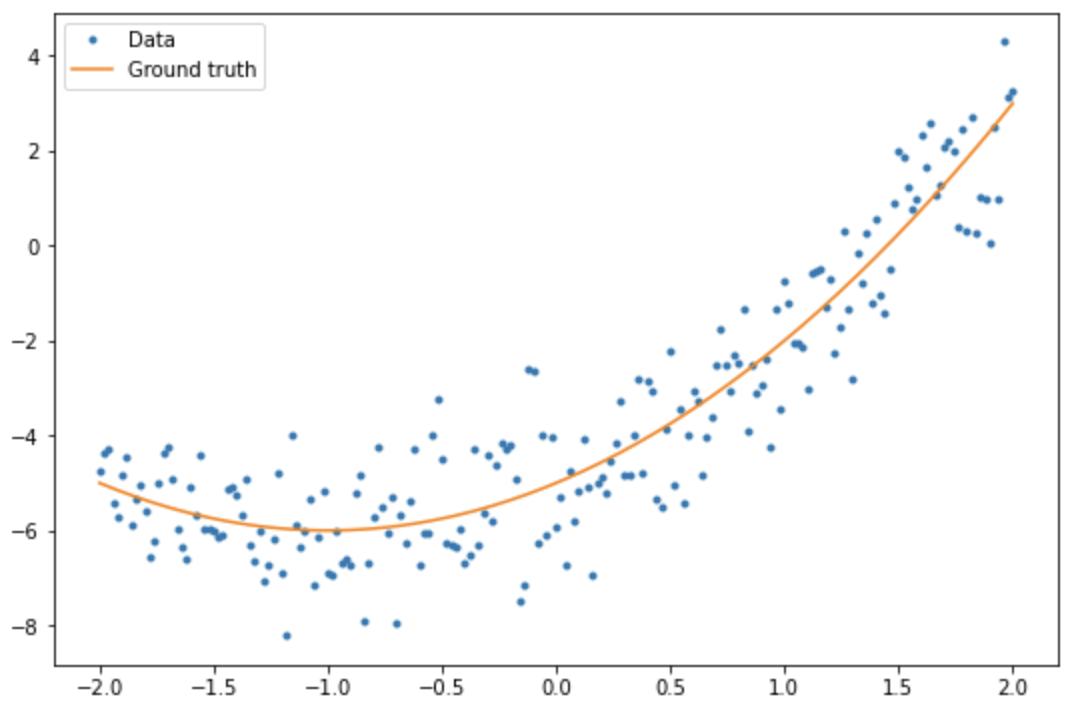
首先，创建一些示例数据。这就产生了一个松散地遵循二次曲线的点云:

import matplotlib
from matplotlib import pyplot as plt

matplotlib.rcParams['figure.figsize'] = [9, 6]

x = tf.linspace(-2, 2, 201)
x = tf.cast(x, tf.float32)

def f(x):
  y = x**2 + 2*x - 5
  return y

y = f(x) + tf.random.normal(shape=[201])

plt.plot(x.numpy(), y.numpy(), '.', label='Data')
plt.plot(x, f(x),  label='Ground truth')
plt.legend();

创建模型:

class Model(tf.keras.Model):
  def __init__(self, units):
    super().__init__()
    self.dense1 = tf.keras.layers.Dense(units=units,
                                        activation=tf.nn.relu,
                                        kernel_initializer=tf.random.normal,
                                        bias_initializer=tf.random.normal)
    self.dense2 = tf.keras.layers.Dense(1)

  def call(self, x, training=True):
    # For Keras layers/models, implement `call` instead of `__call__`.
    x = x[:, tf.newaxis]
    x = self.dense1(x)
    x = self.dense2(x)
    return tf.squeeze(x, axis=1)

这里：

• tf.keras.layers.Dense构建一个神经层，units传入的参数是输出的维度，kernel_initializer和bias_initializer这里用tf.random.normal各生成一组随机正态分布的向量
• tf.squeeze的作用是移除一维向量

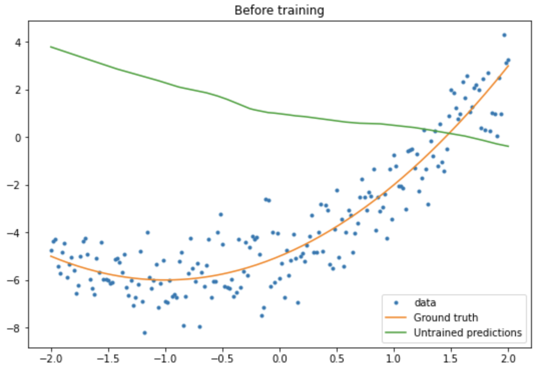
model = Model(64)

plt.plot(x.numpy(), y.numpy(), '.', label='data')
plt.plot(x, f(x),  label='Ground truth')
plt.plot(x, model(x), label='Untrained predictions')
plt.title('Before training')
plt.legend();

写一个基本的training loop:

variables = model.variables

optimizer = tf.optimizers.SGD(learning_rate=0.01)

for step in range(1000):
  with tf.GradientTape() as tape:
    prediction = model(x)
    error = (y-prediction)**2
    mean_error = tf.reduce_mean(error)
  gradient = tape.gradient(mean_error, variables)
  optimizer.apply_gradients(zip(gradient, variables))

  if step % 100 == 0:
    print(f'Mean squared error: {mean_error.numpy():0.3f}')

Mean squared error: 39.156
Mean squared error: 1.100
Mean squared error: 1.070
Mean squared error: 1.052
Mean squared error: 1.039
Mean squared error: 1.030
Mean squared error: 1.023
Mean squared error: 1.017
Mean squared error: 1.012
Mean squared error: 1.008

plt.plot(x.numpy(),y.numpy(), '.', label="data")
plt.plot(x, f(x),  label='Ground truth')
plt.plot(x, model(x), label='Trained predictions')
plt.title('After training')
plt.legend();

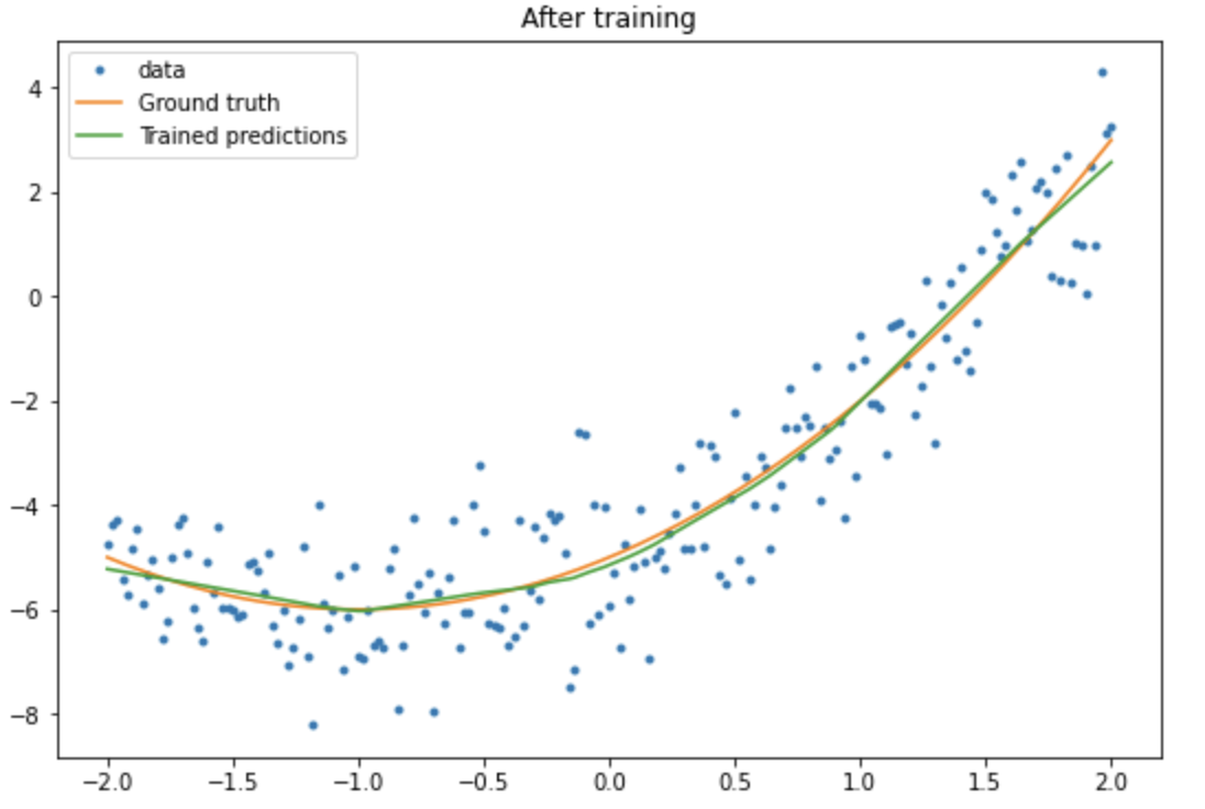
以上便是用一个拟合的过程，这里的训练过程还是以Keras为主。
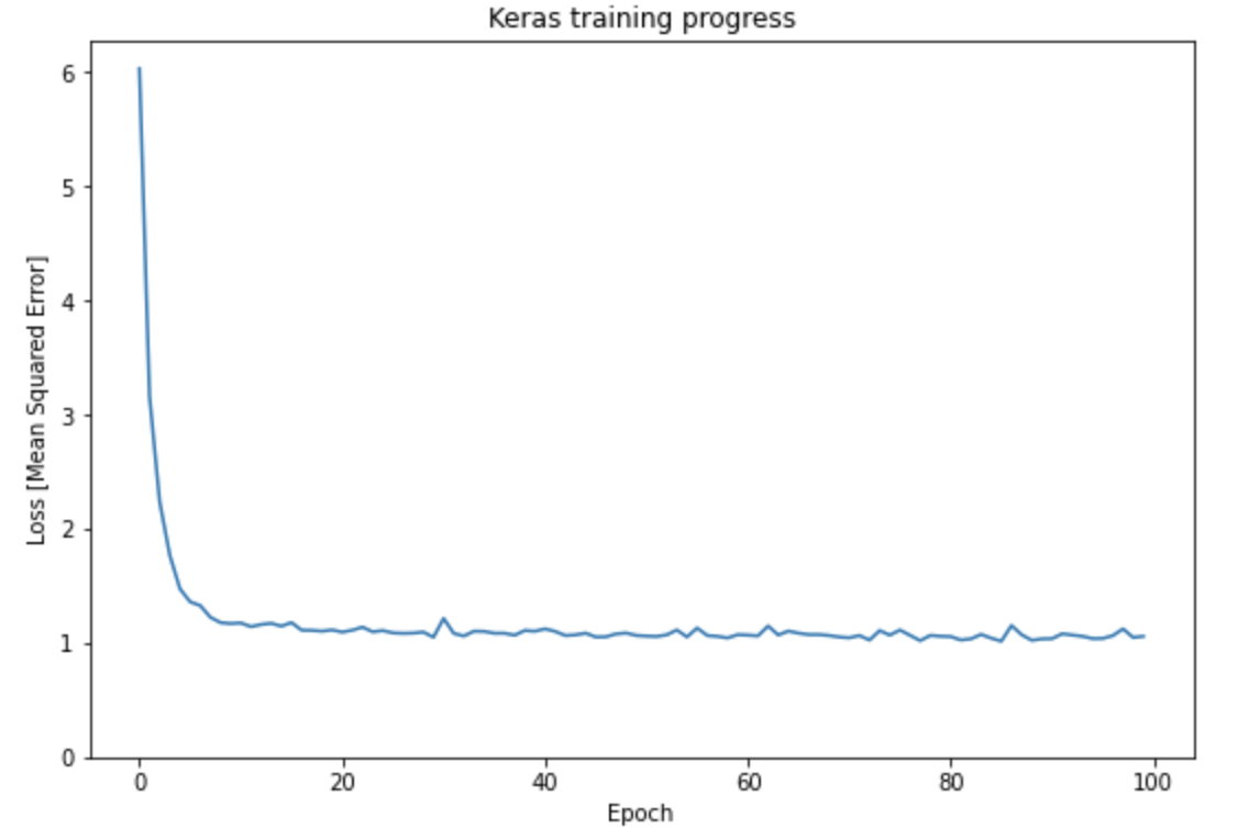
可以用Model.compile 和Model.fit实现自己的training loop。

new_model = Model(64)

new_model.compile(
    loss=tf.keras.losses.MSE,
    optimizer=tf.optimizers.SGD(learning_rate=0.01))

history = new_model.fit(x, y,
                        epochs=100,
                        batch_size=32,
                        verbose=0)

model.save('./my_model')

INFO:tensorflow:Assets written to: ./my_model/assets

plt.plot(history.history['loss'])
plt.xlabel('Epoch')
plt.ylim([0, max(plt.ylim())])
plt.ylabel('Loss [Mean Squared Error]')
plt.title('Keras training progress');