RCNN系列——RCNN、fast RCNN、FasterRCNN

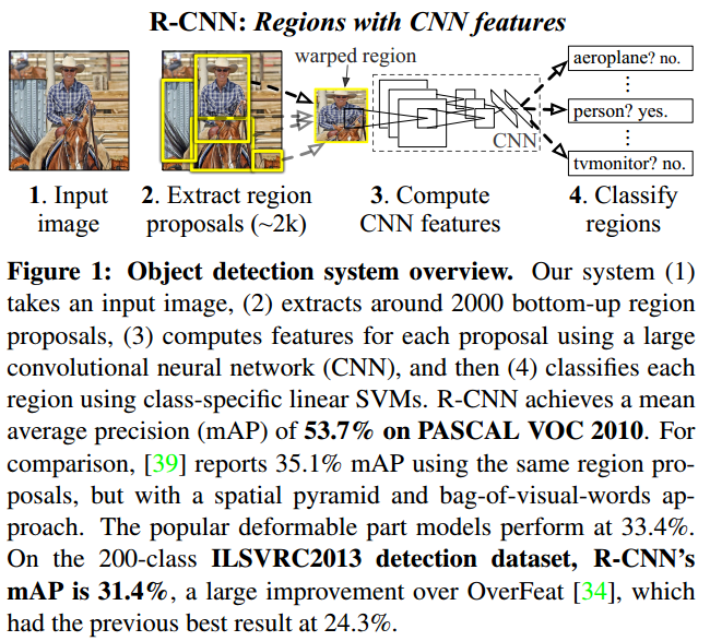
一、Rich feature hierarchies for accurate object detection and semantic segmentation

论文地址：http://openaccess.thecvf.com/content_cvpr_2014/papers/Girshick_Rich_Feature_Hierarchies_2014_CVPR_paper.pdf

引用量：11000+

具体流程有如下三步：

A.利用selective search方法选取大约2000个左右的region proposal(图像上框出来的长方形框)。

B.对每个proposal通过CNN得到feature。

C.然后用SVM对feature分类，得到每个proposal的类别。

整体框架

 

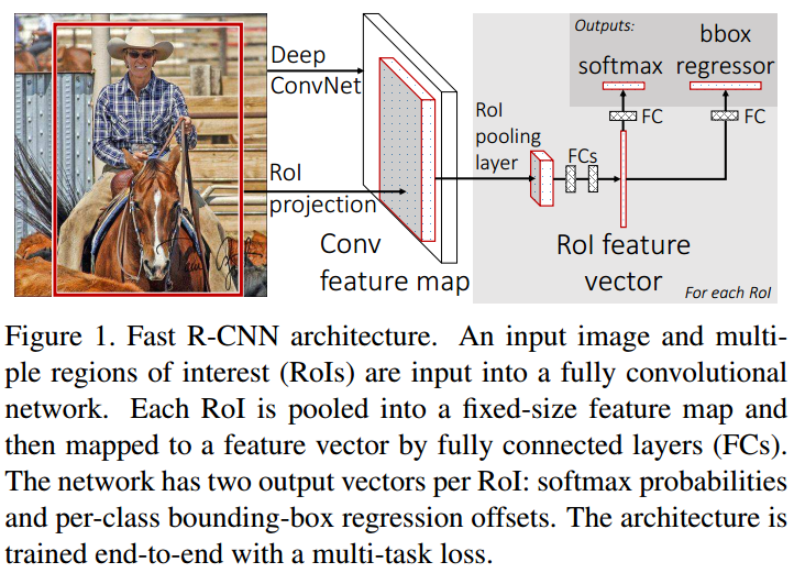
二、Fast R-CNN

论文地址：http://openaccess.thecvf.com/content_iccv_2015/papers/Girshick_Fast_R-CNN_ICCV_2015_paper.pdf

引用量：8000+

R-CNN因为每个region都需要通过CNN处理得到feature，故而有很多重复计算，严重影响了速度。

具体处理步骤：

A.先用CNN处理图像得到整个图像对应的feature，先将一张图像送入网络，而后将候选区域映射到图像feature，得到region of interest，这些候选区域的前几层特征不需要再重复计算。

B.将选出来的region映射到feature，得到每个region对应的feature，称之为region_feature。

C.利用ROI pooling对每一个region_feature统一为固定大小的feature，称之为fixed_feature。

D.通过全连接层处理每一个fixed_feature，在进行分类和回归。

整体框架：

ROI pooling layer:可参考 https://www.cnblogs.com/AntonioSu/p/11945892.html

   

三、Faster R-CNN: Towards Real-Time Object Detection with Region Proposal Networks

论文地址：http://papers.nips.cc/paper/5638-faster-r-cnn-towards-real-time-object-detection-with-region-proposal-networks.pdf

引用量：15000+

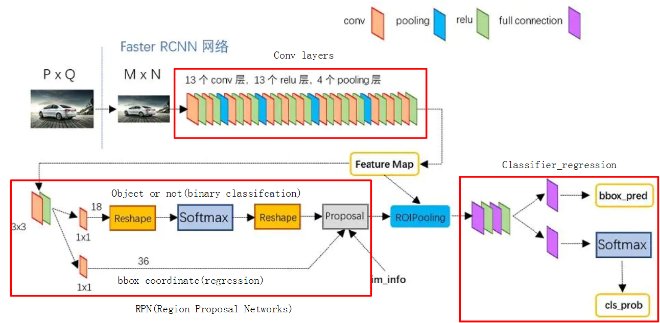
1.网络整体框架

 

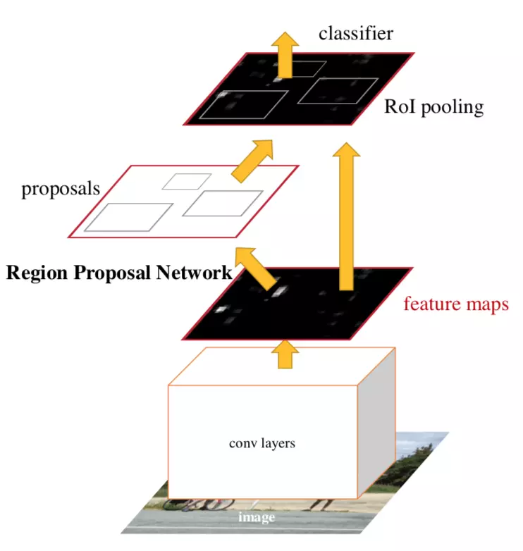
对上图先做一个简单的介绍

conv layers：用于提取图像的特征。输入是图片，输出是feature maps。

RPN网络：用于产生proposal。其中一支是判断前景or背景，一支是对位置坐标的初步回归。输入是feature maps，输出是proposal的位置偏移和类别(前景or背景)。

ROI pooling：统一大小不同的feature。将RPN的得到的proposal映射的feature maps，得到每个proposal的feature，而后对每个大小不同的proposal feature统一为大小相同的feature。

classifier：产生真正的类别和坐标。经过全连接层处理ROI pooling产生的feature，而后回归proposal在图像中的精确位置，输出proposal对应的类别。

 

2.具体框架

1) conv layers

输入图片是MxN，经过conv  layers，下采样16次，得到WxHx512(W=M/16,H=N/16)大小的feature maps。

2) RPN网络

输入：是conv layers产生的feature maps。对应feature maps的维度是WxHx512。

目的：生成proposal。操作方式是通过引入anchor，而后过滤得到proposal。

 

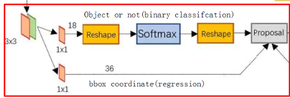
分类网络(object or not):是将WxHx512通过1x1的卷积核转化为WxHx18=WxHx9x2(其中9表示每个特征点取9种形状的方框，2表示前景和背景)。

回归网络(bbox coordinate):是将WxHx512通过1x1的卷积核转化为WxHx36=WxHx9x4(9同上，4是对应的4个坐标偏移值△x, △y, △w, △h)。

其中RPN网络会舍弃超出边界的anchor，利用nms过滤anchor，去除背景anchor，最后生成大概300左右的anchor，称之为proposal。

A.proposal

layer {  
  name: 'proposal'  
  type: 'Python'  
  bottom: 'rpn_cls_prob_reshape' #[1,18,40,60]==> [batch_size, channel，height，width]Caffe的数据格式，anchor box分类的概率
  bottom: 'rpn_bbox_pred'  # 记录训练好的四个回归值x,y,w,h
  bottom: 'im_info'  
  top: 'rpn_rois'  
  python_param {  
    module: 'rpn.proposal_layer'  
     layer: 'ProposalLayer'  
     param_str: "'feat_stride': 16 \n'scales': !!python/tuple [4, 8, 16, 32]"
   }  
 }

 

其中rpn_bbox_pred 是WxHx9个anchor box加上对应的偏移值△x, △y, △w, △h，得到更加准确的bounding box。

其中rpn_cls_prob_reshape是由回归网络(bbox coordinate)得到的前景or背景的概率。

 

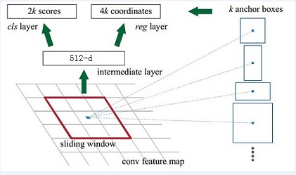
B.Anchor box

在特征图(feature maps)上的每一个点取9个候选区域（3个不同尺度，3个不同长宽比），称之为anchor box，亦称为ROI(region of interest)。

 

 3)ROI pooling

其中 feature maps的维度是WxHx512。

RPN的得到的300个proposal，每个proposal的大小各不相同。

将proposal映射到feature maps，得到proposal的feature，proposal_feature的维度为300*512*x*y，其中每个proposal的x和y都不相同。

最后通过ROI pooling将300*512*x*y转化为统一的维度：300*512*7*7。

具体ROIPooling详细过程参见：https://www.cnblogs.com/AntonioSu/p/11945892.html

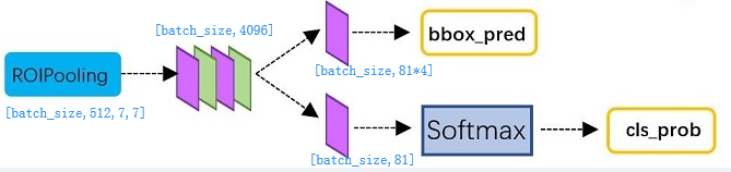
4)Classifer_regression

对ROI pooling产生的tensor(300*512*7*7),其中300是proposal的个数，相当于batch_size=300，经过全连接层，分两支得到bbox_pred=[batch_size,81*4]和cls_prob=[batch_size,81]。

bbox_pred表示对应的bbox的坐标，cls_prob表示对应的类别。

 

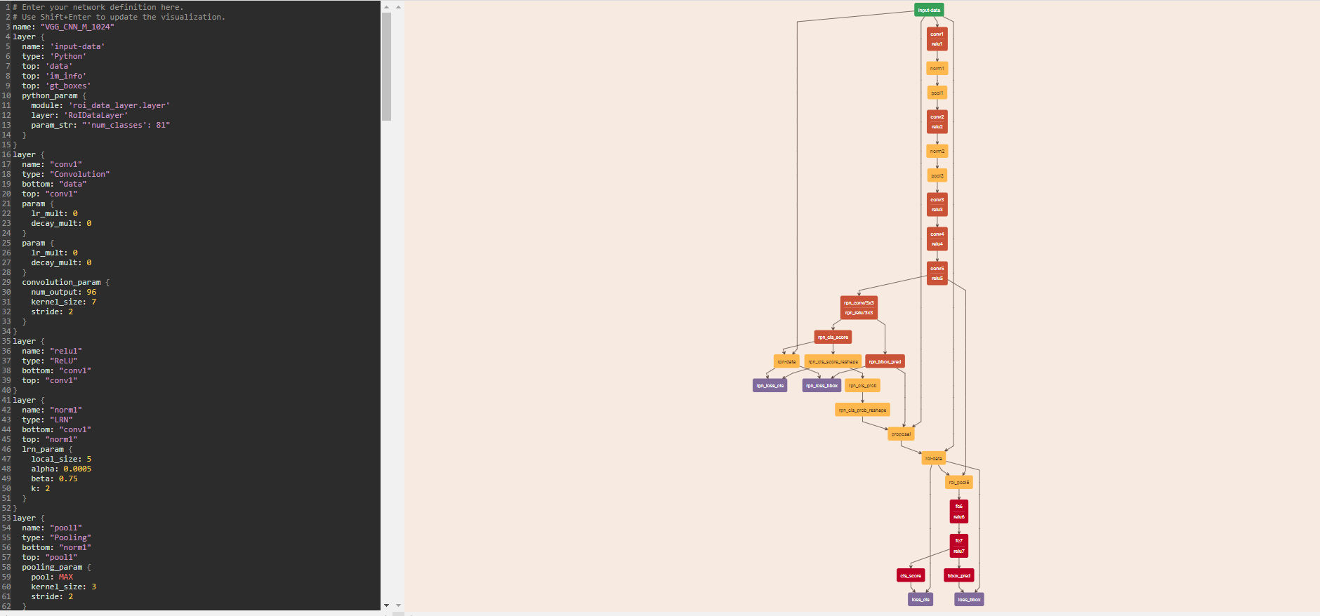
3.数据流图

利用对.prototxt可视化工具http://ethereon.github.io/netscope/#/editor。

具体步骤：将https://github.com/rbgirshick/py-faster-rcnn/blob/master/models/coco/VGG_CNN_M_1024/faster_rcnn_end2end/train.prototxt文件输入到http://ethereon.github.io/netscope/#/editor，而后shift+enter，可以查看具体的数据流。

展示结果如下：