[Machine Learning] Diagnosing Bias vs. Variance
In this section we examine the relationship between the degree of the polynomial d and the underfitting or overfitting of our hypothesis.
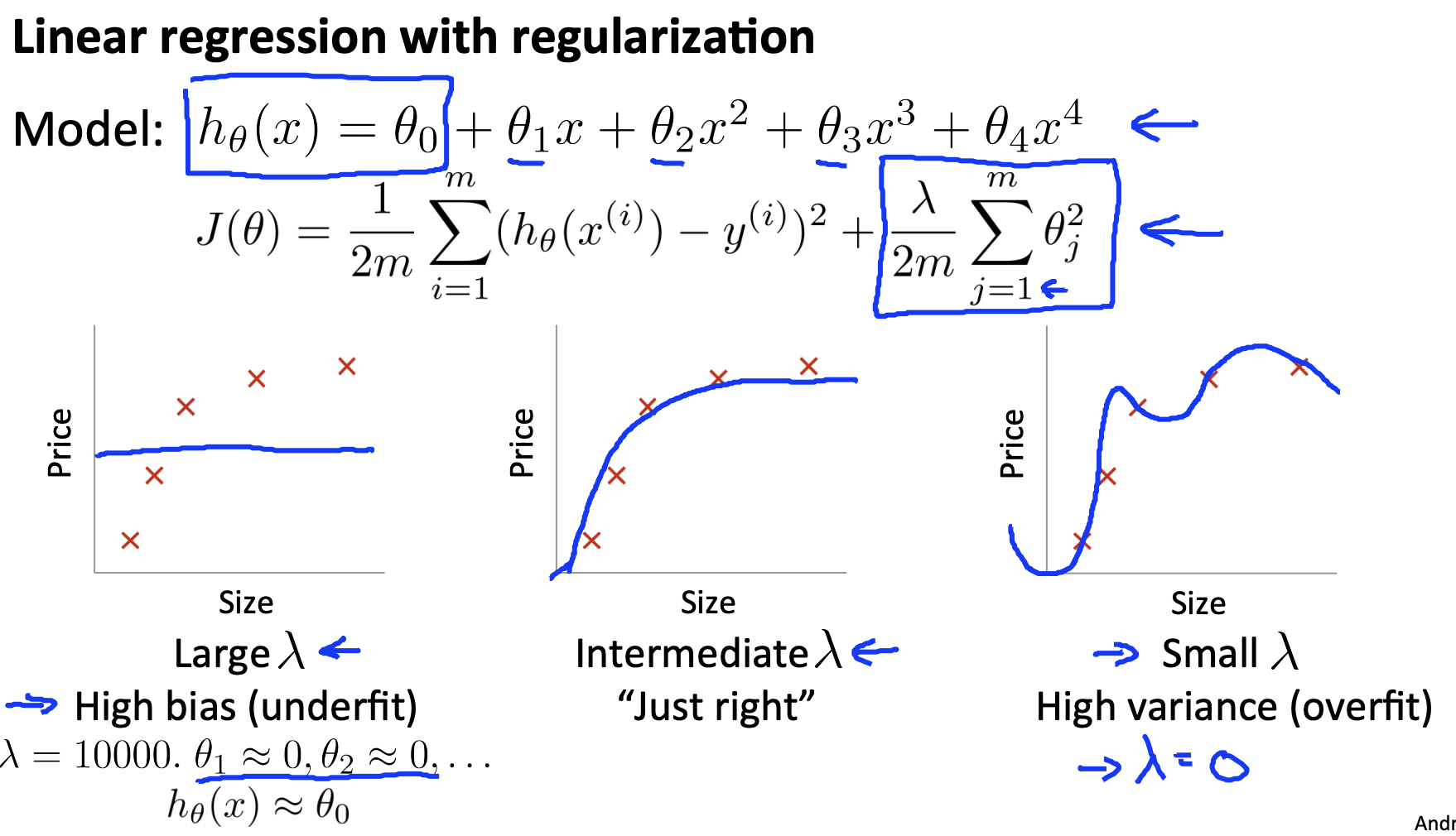
- We need to distinguish whether bias or variance is the problem contributing to bad predictions.
- High bias is underfitting and high variance is overfitting. Ideally, we need to find a golden mean between these two.
The training error will tend to decrease as we increase the degree d of the polynomial.
At the same time, the cross validation error will tend to decrease as we increase d up to a point, and then it will increase as d is increased, forming a convex curve.

Our decision process can be broken down as follows:
- Getting more training examples: Fixes high variance
- Trying smaller sets of features: Fixes high variance
- Adding features: Fixes high bias
- Adding polynomial features: Fixes high bias
- Decreasing λ: Fixes high bias
- Increasing λ: Fixes high variance.
Diagnosing Neural Networks
- A neural network with fewer parameters is prone to underfitting. It is also computationally cheaper.
- A large neural network with more parameters is prone to overfitting. It is also computationally expensive. In this case you can use regularization (increase λ) to address the overfitting.
Using a single hidden layer is a good starting default. You can train your neural network on a number of hidden layers using your cross validation set. You can then select the one that performs best.
Model Complexity Effects:
- Lower-order polynomials (low model complexity) have high bias and low variance. In this case, the model fits poorly consistently.
- Higher-order polynomials (high model complexity) fit the training data extremely well and the test data extremely poorly. These have low bias on the training data, but very high variance.
- In reality, we would want to choose a model somewhere in between, that can generalize well but also fits the data reasonably well.

 浙公网安备 33010602011771号