Introduction to graph theory（图论简介）

Overview

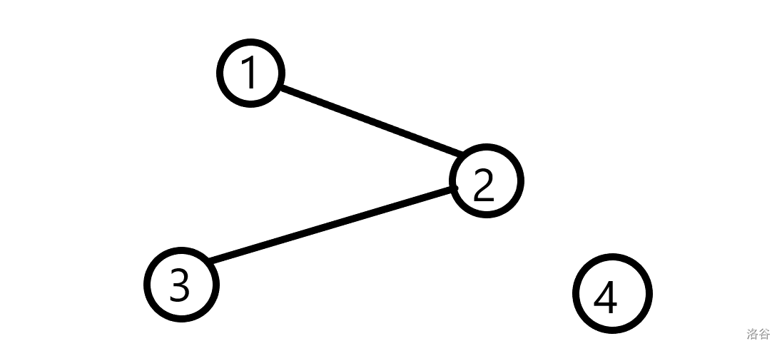
Graph is a kind of data struction. It's very useful, it can descripe the relationship of a lot things. In the life, we always see the graph, such as the traffic graph. For instance, this is a graph.

There are 4 nodes in this graph. And there is two edges in this graph. It is a undirected graph.

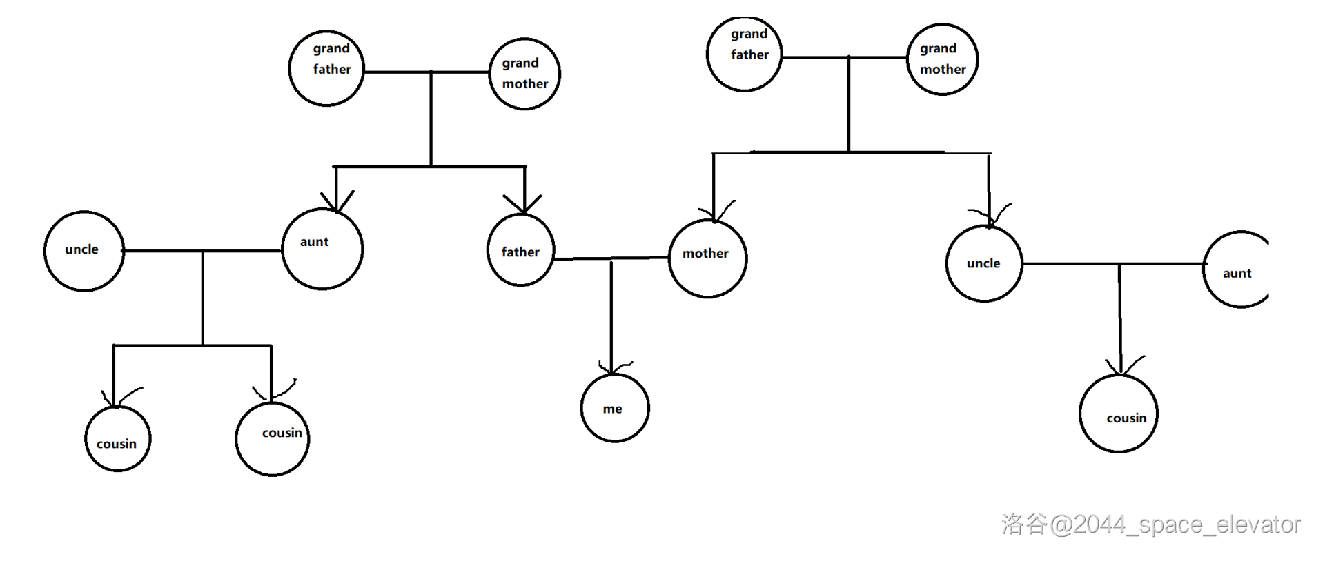
Of course, we have directed graph too. This is directed graph about my genealogy.

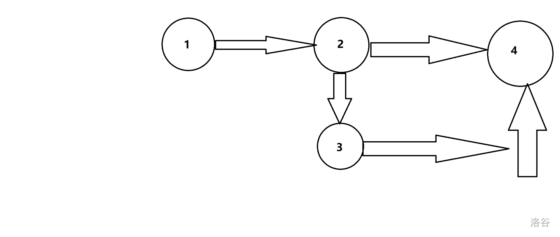
This is a directed graph too.

Now, you know what a graph is, and then, I will introduction to how to denote a graph.

Denote a graph

There are two representation methods to denote a graph. One is matrix, and the other one is adjacency table, adjacency table is a little complex, in this article, I only introduction matrix representation method.

Undirected graph

For instance, we denote the graph of picture 1, this the matrix of picture 1:
$$
\begin{bmatrix}
0 & 1 & 0 & 0\
1 & 0 & 1 & 0\
0 & 1 & 0 & 0\
0 & 0 & 0 & 0
\end{bmatrix}
$$
In matrix, if node $a$ and node $b$ are connected, $A_{ab},A_{ba}=1$, otherwise $A_{ab},A_{ba}=0$

In picture 1, there are $2$ edges, they are:

• $1 \operatorname{and} 2$
• $2 \operatorname{and} 3$

So:

• $A_{12},A_{21}=1$
• $A_{23},A_{32}=1$

Directed graph

There are new rules for representing directed graphs in matrices:

• If $a \to b$, $A_{ab}=1$
• If $b \to a$, $A_{ba}=1$

For instance, we denote the graph of picture 3.

There are $4$ edges in picture 3, they are:

• $1\to 2$
• $2\to 3$
• $3\to 4$
• $2\to 4$

So, the matrix of picture 3 like this:
$$
\begin{bmatrix}
0 & 1 & 0 & 0\
0 & 0 & 1 & 1\
0 & 0 & 0 & 1\
0 & 0 & 0 & 0
\end{bmatrix}
$$

Weighted graph

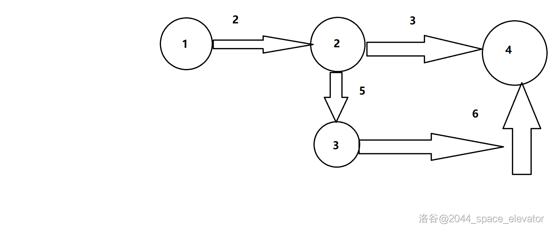
This is a weighted graph.

If node $a$ and $b$ are connected, and there weight is $k$, this is the representation method of weighted graphs.

• If $a\to b$, $A_{ab} = k$
• If $b\to a$, $A_{ba} = k$
• Otherwise, $A_{ab},A_{ba}=\infty$

The matrix of picture 4:
$$
\begin{bmatrix}
\infty & 2 & \infty & \infty\
\infty & \infty & 5 & 3\
\infty & \infty & \infty & 6\
\infty & \infty & \infty & \infty
\end{bmatrix}
$$

Denote by code

Undirected graph

Let's first define a two-dimensional array. For instance, this is the input of picture 3.

4
1 2
2 3
3 4
2 4

It means, there are $4$ edges in this graph, $1$ and $2$ was connected, $2$ and $3$ was connected, $3$ and $4$ was connected, $2$ and $4$ was connected.

This is the code to record the graph:

#include <iostream>
using namespace std;

bool A[10][10];
int n;

int main()
{
    cin >> n;
    while (n--)
    {
        int node1, node2;
        cin >> node1 >> node2;
        A[node1][node2] = 1;
        A[node1][node2] = 1;
    }
    return 0;
}

Directed graph

This is the code of denote directed graph.

#include <iostream>
using namespace std;

bool A[10][10];
int n;

int main()
{
    cin >> n;
    while (n--)
    {
        int node1, node2;
        cin >> node1 >> node2;
        A[node1][node2] = 1;
    }
    return 0;
}

Weighted graph

This is the code of denote directed graph:

#include <iostream>
using namespace std;
#define oo 123456
int A[10][10];
int n;

int main()
{
    // init
    cin >> n;
    for (int i = 1; i <= 9; i++)
    {
        for (int j = 1; j <= 9; j++)
        {
            A[i][j] = oo;
        }
    }
    while (n--)
    {
        int node1, node2, weight;
        cin >> node1 >> node2 >> weight;
        A[node1][node2] = weight;
    }
    return 0;
}

Search algorithm

There are two kinds of search algorithms graphs: depth first search(dfs) and breadth first search(bfs), dfs is easier than bfs, but dfs is very slow.

In this article, we call the first node of graph "root", such as in picture 4, the "root" is node 1.

Depth first search

You maybe have learnt the backtracking algorithm, this is template code for backtracking:

void backtracking(...)
{
    if (Marginal Condition)
    {
        Save result
        return;
    }
    for (int i = startIndex; i <= n; i++)
    {
        Record vales
        backtracking(...);
        Delet vales
    }
}

Backtracking is a kind of depth first search., the dfs of graph is very like backtracking, this is the template code of dfs of graph.:

bool vis[N]; // Tag
int n; // node number
void dfs(int node)
{
    if (node == n)
    {
        // output path
        return;
    }
    for (int i = 1; i <= n; i++)
    {
        if ((A[i][node] == 1 || A[node][i] == 1) && !vis[i])
        {
            vis[i] = 1;
            dfs(i);
            vis[i] = 0;
        }
    }
}

Breadth first search

In fact, breadth first search (bfs) equivalent to level traversal, such as, this is the bfs of picture 3, we set the root node is 1.

We need a queue. First, we put the root node in the queue:

queue:
1
path:

And then, we record node 1, and put all children of node 1 in the queue:

queue:
2
path:
1

Next, we record node 2, and put all children of node 1 in the queue:

queue:
3 4
path:
1 2

Finally, we record node 3 and node 4, put all children of them in the queue:

queue:
path:
1 2 4 3

Node 4 has no children, the children of node 3 has a child (node 4), but it has recorded.

So this is the temple code of bfs:

#include <queue> // We need the queue
int A[N][N];
bool vis[N]; // Has visited?
void bfs()
{
    queue<int> path;
    path.push(/*root node*/);
    vis[/*root node*/] = true;
    while (!path.empth())
    {
        int node = path.front();
        /*record node*/
        path.pop();
        for (int i = 1; i <= N; i++)
        {
            if ((A[node][i] || A[i][node]) && !vis[i])
            {
                path.push(i);
                vis[i] = true;
            }
        }
    }
}

Summarize

Of course, there are many special graph, such as: binary tree, red-black tree, cyclic graph and so on. This article introduces the basic knowledge of graphs.

If this article is helpful to you, please give it a positive review. Thank you!