作业3

任务：对数据中中国0-14岁人口比例与年份的关系进行回归分析，不借助网络自己动手构建一个线性回归系统，学习数据中的分布并完成2018-2022年人口比例走势的预测（即2013-2022年的数据为测试集，之前的数据为训练集），至少使用MSE指标评估模型在测试数据集上的性能。学习框架可以采用最小二乘算法，梯度下降算法，岭回归算法等。

1.最小二乘法

import numpy as np
import pandas as pd
import matplotlib.pyplot as plt

# 数据导入与预处理
import pandas as pd
# 数据导入，跳过前4行（World Bank 数据集常有的说明性行）
data = pd.read_csv('本地文件/API_4_DS2_en_csv_v2_2807.csv', skiprows=4)
# 筛选出中国的数据，选择'Population ages 0-14 (% of total population)'的指标
china_data = data[(data['Country Name'] == 'China') & 
                  (data['Indicator Name'] == 'Population ages 0-14 (% of total population)')]
# 转换年份列为行，过滤掉非数字列
china_data = china_data.melt(id_vars=['Country Name', 'Country Code', 'Indicator Name', 'Indicator Code'], 
                             var_name='Year', value_name='Population 0-14 Age %')
# 确保'Year'列只包含数字，并去除非年份的行
china_data = china_data[china_data['Year'].str.isdigit()]
# 将'Year'列转换为整数
china_data['Year'] = china_data['Year'].astype(int)
# 去除缺失值
china_data = china_data.dropna(subset=['Population 0-14 Age %'])
# 查看处理后的数据
print(china_data.head())


# 训练集和测试集划分
# 只保留2000年之后的数据
china_population_data_recent = china_data[china_data['Year'] >= 2000]
# 将训练集设置为2000-2012，测试集为2013-2022
train_data = china_population_data_recent[china_population_data_recent['Year'] <= 2012]
test_data = china_population_data_recent[china_population_data_recent['Year'] > 2012]
# 特征为年份，目标为0-14岁人口比例
X_train = train_data[['Year']]
y_train = train_data['Population 0-14 Age %']
X_test = test_data[['Year']]
y_test = test_data['Population 0-14 Age %']

# 最小二乘法
from sklearn.linear_model import LinearRegression
from sklearn.metrics import mean_squared_error

# 创建并训练线性回归模型
model = LinearRegression()
model.fit(X_train, y_train)

# 进行预测
y_pred = model.predict(X_test)

# 计算均方误差(MSE)
mse = mean_squared_error(y_test, y_pred)
print(f"Mean Squared Error (MSE) on Test Data: {mse}")

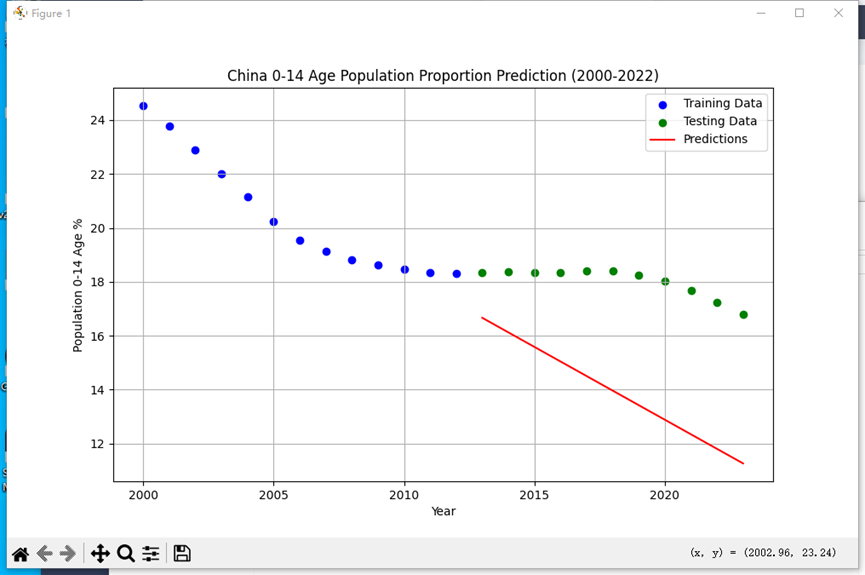
import matplotlib.pyplot as plt

# 绘制预测结果与实际数据
plt.figure(figsize=(10, 6))
plt.scatter(X_train, y_train, color='blue', label='Training Data')
plt.scatter(X_test, y_test, color='green', label='Testing Data')
plt.plot(X_test, y_pred, color='red', label='Predictions')
plt.xlabel('Year')
plt.ylabel('Population 0-14 Age %')
plt.title('China 0-14 Age Population Proportion Prediction (2000-2022)')
plt.legend()
plt.grid(True)
plt.show()

2.梯度下降算法，岭回归算法

import numpy as np
import pandas as pd
import matplotlib.pyplot as plt
from sklearn.model_selection import train_test_split
from sklearn.linear_model import Ridge
from sklearn.metrics import mean_squared_error

# 数据导入
data = pd.read_csv('本地文件/API_4_DS2_en_csv_v2_2807.csv', skiprows=4)

# 筛选中国的数据，选择'Population ages 0-14 (% of total population)'的指标
china_data = data[(data['Country Name'] == 'China') & 
                  (data['Indicator Name'] == 'Population ages 0-14 (% of total population)')]

# 转换年份列为行，过滤掉非数字列
china_data = china_data.melt(id_vars=['Country Name', 'Country Code', 'Indicator Name', 'Indicator Code'], 
                             var_name='Year', value_name='Population 0-14 Age %')

# 确保'Year'列只包含数字，并去除非年份的行
china_data = china_data[china_data['Year'].str.isdigit()]

# 将'Year'列转换为整数
china_data['Year'] = china_data['Year'].astype(int)

# 去除缺失值
china_data = china_data.dropna(subset=['Population 0-14 Age %'])

# 特征变量（年份）和目标变量（人口比例）
X = china_data[['Year']].values
y = china_data['Population 0-14 Age %'].values

# 划分训练集和测试集，80%为训练集，20%为测试集
X_train, X_test, y_train, y_test = train_test_split(X, y, test_size=0.2, random_state=42)

# ---- 1. 梯度下降法实现线性回归 ---- #
# 标准化数据
X_train_scaled = (X_train - np.mean(X_train)) / np.std(X_train)
X_test_scaled = (X_test - np.mean(X_train)) / np.std(X_train)

# 添加偏置项
X_b_train = np.c_[np.ones((len(X_train_scaled), 1)), X_train_scaled]
X_b_test = np.c_[np.ones((len(X_test_scaled), 1)), X_test_scaled]

# 初始化参数
theta = np.random.randn(2, 1)  # 两个参数：权重和偏置
learning_rate = 0.01
n_iterations = 1000
m = len(X_train_scaled)

# 梯度下降算法
for iteration in range(n_iterations):
    gradients = 2/m * X_b_train.T.dot(X_b_train.dot(theta) - y_train.reshape(-1, 1))
    theta = theta - learning_rate * gradients

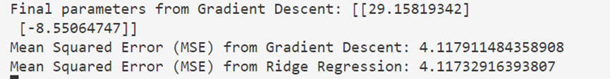
# 打印最终的参数
print(f"Final parameters from Gradient Descent: {theta}")

# 预测结果
y_pred_gd = X_b_test.dot(theta)

# 计算MSE
mse_gd = mean_squared_error(y_test, y_pred_gd)
print(f"Mean Squared Error (MSE) from Gradient Descent: {mse_gd}")

# ---- 2. 岭回归实现 ---- #
# 创建并训练岭回归模型
ridge_model = Ridge(alpha=1.0)  # alpha 是正则化强度，值越大正则化越强
ridge_model.fit(X_train, y_train)

# 进行预测
y_pred_ridge = ridge_model.predict(X_test)

# 计算MSE
mse_ridge = mean_squared_error(y_test, y_pred_ridge)
print(f"Mean Squared Error (MSE) from Ridge Regression: {mse_ridge}")

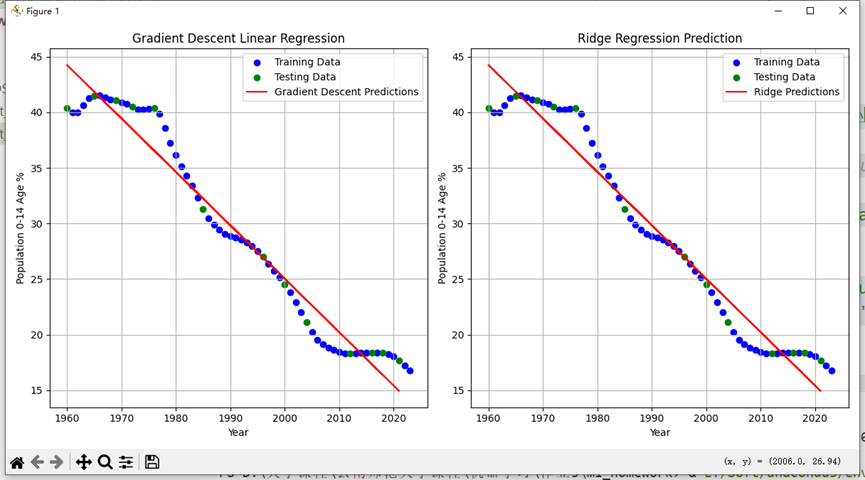
# ---- 3. 可视化梯度下降与岭回归的预测结果 ---- #
plt.figure(figsize=(12, 6))

# 梯度下降法的预测结果
plt.subplot(1, 2, 1)
plt.scatter(X_train, y_train, color='blue', label='Training Data')
plt.scatter(X_test, y_test, color='green', label='Testing Data')
plt.plot(X_test, y_pred_gd, color='red', label='Gradient Descent Predictions')
plt.xlabel('Year')
plt.ylabel('Population 0-14 Age %')
plt.title('Gradient Descent Linear Regression')
plt.legend()
plt.grid(True)

# 岭回归的预测结果
plt.subplot(1, 2, 2)
plt.scatter(X_train, y_train, color='blue', label='Training Data')
plt.scatter(X_test, y_test, color='green', label='Testing Data')
plt.plot(X_test, y_pred_ridge, color='red', label='Ridge Predictions')
plt.xlabel('Year')
plt.ylabel('Population 0-14 Age %')
plt.title('Ridge Regression Prediction')
plt.legend()
plt.grid(True)

plt.tight_layout()
plt.show()