机器学习及其应用

Task 1. Pandas, Numpy, Matplotlib (3 points)#

Subproblem 1.1 (1 point)#

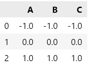
Write a function, which takes a pandas DataFrame df and substract the mean value and divide by standard deviation each column.

Copy
import pandas as pd
import numpy as np
import matplotlib.pyplot as plt

Copy
df = pd.DataFrame({'A':[1,2,3], 'B':[1,2,3], 'C':[1,2,3]})`
def normalize(df):
    """Shift by mean and scale by standard deviation each column of a DataFrame.

    Parameters
    ----------
    df : pandas.Dataframe, shape = (n_rows, n_cols)
        The Dataframe, the columns of which to normalize.

    Returns
    ----------
    out : Dataframe, shape = (n_rows, n_cols)
        The final column-centered Dataframe.
    """
    n_rows, n_cols = df.shape

    ### BEGIN Solution (do not delete this comment)
    df_bak = df
    for col_name in df_bak:
        mean = df_bak[col_name].mean()
        std = df_bak[col_name].std()
        df_bak[col_name] = df_bak[col_name].map(lambda x: (x-mean)/std)  
    out = df_bak
    ### END Solution (do not delete this comment)

    return out

Copy
print("EXPECTED OUTPUT FORMAT\n")
normalize(df)

Subproblem 1.2 (1 point)#

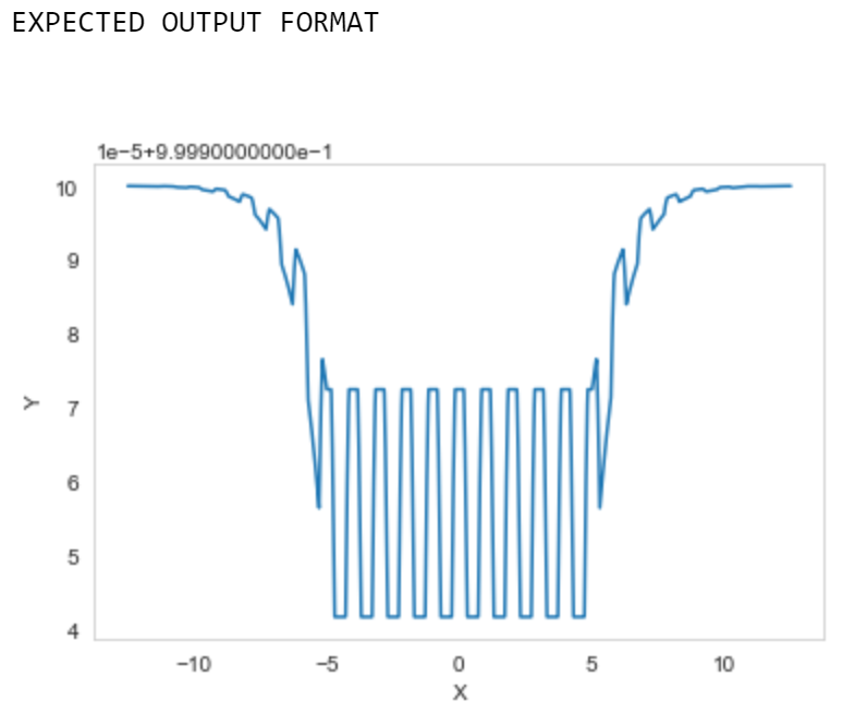
Plot the following fancy function:
$$\begin{equation} f(x) = \sigma\bigl( \max{x + 5, 0} + \max{5 - x, 0} + \max{\min{\cos(2 x \pi), \tfrac12}, -\tfrac14} \bigr) , \end{equation}$$
where $\sigma(x) = (1+e^{-x})^{-1}$ is the sigmoid function.

Plot your function for the x-values ranging from $-12.5$ to $12.5$

Copy
def fancy_function(x):
    """Compute some fancy function.
    
    Parameters
    ----------
    X : array, 1 dimendional, shape=(n_samples,)
        The array argument values.

    Returns
    -------
    y : array, 1 dimendional, shape=(n_samples,)
        The values of the fancy function.
    """
    ### BEGIN Solution
    # x = np.arange(-12.5,12.5,0.01)
    a = np.array(x)
    np.clip(a,-12.5,12.5,out=a)
    sigma_x = np.maximum(a+5,0)+np.maximum(5-a,0)+np.maximum(np.minimum(np.cos(2*a*np.pi),0.5),-0.25)
    out = (1 + np.exp(-sigma_x))**(-1)
    # print(out)
    ### END Solution
    
    return out

Plot fancy_function(x)#

Copy
print("EXPECTED OUTPUT FORMAT\n")
### BEGIN Solution
import matplotlib.pyplot as plt
import seaborn as sns
sns.set_style('whitegrid')
%matplotlib inline
x = np.arange(-12.5,12.5,0.01)
# Simple plot
x = x
y = fancy_function(x)
plt.plot(x, y,)
plt.xlabel('X')
plt.ylabel('Y')
plt.grid(None)
### END Solution
plt.show()

Task 4. Boosting (2 points)#

Copy
%matplotlib inline

import numpy as np
import matplotlib.pyplot as plt
from matplotlib.colors import ListedColormap

from sklearn.datasets import make_moons
from sklearn.model_selection import train_test_split
from sklearn.ensemble import AdaBoostClassifier

Boosting Machines (BM) is a family of widely popular and effective methods for classification and regression tasks. The main idea behind BMs is that combining weak learners, which perform slightly better than random, can result in strong learning models.

AdaBoost utilizes the greedy training approach: firstly, we train the weak learners (they are later called base_classifiers) on the whole dataset and in the next iterations we train the model on the samples, on the which the previous models have performed poorly. This behavior is achieved by reweighting the training samples during each algorithm's step.

The task:#

In this exercise you will be asked to implement one of the earlier variants of BMs - AdaBoost and compare it to the already existing sklearn implementation (in the sklearn function do not forget to use algorithm=SAMME). The key steps are:

• Complete the .fit method of Boosting class

• Complete the .predict method of Boosting class

The pseudocode for AdaBoost can be found in lectures and seminar 7.

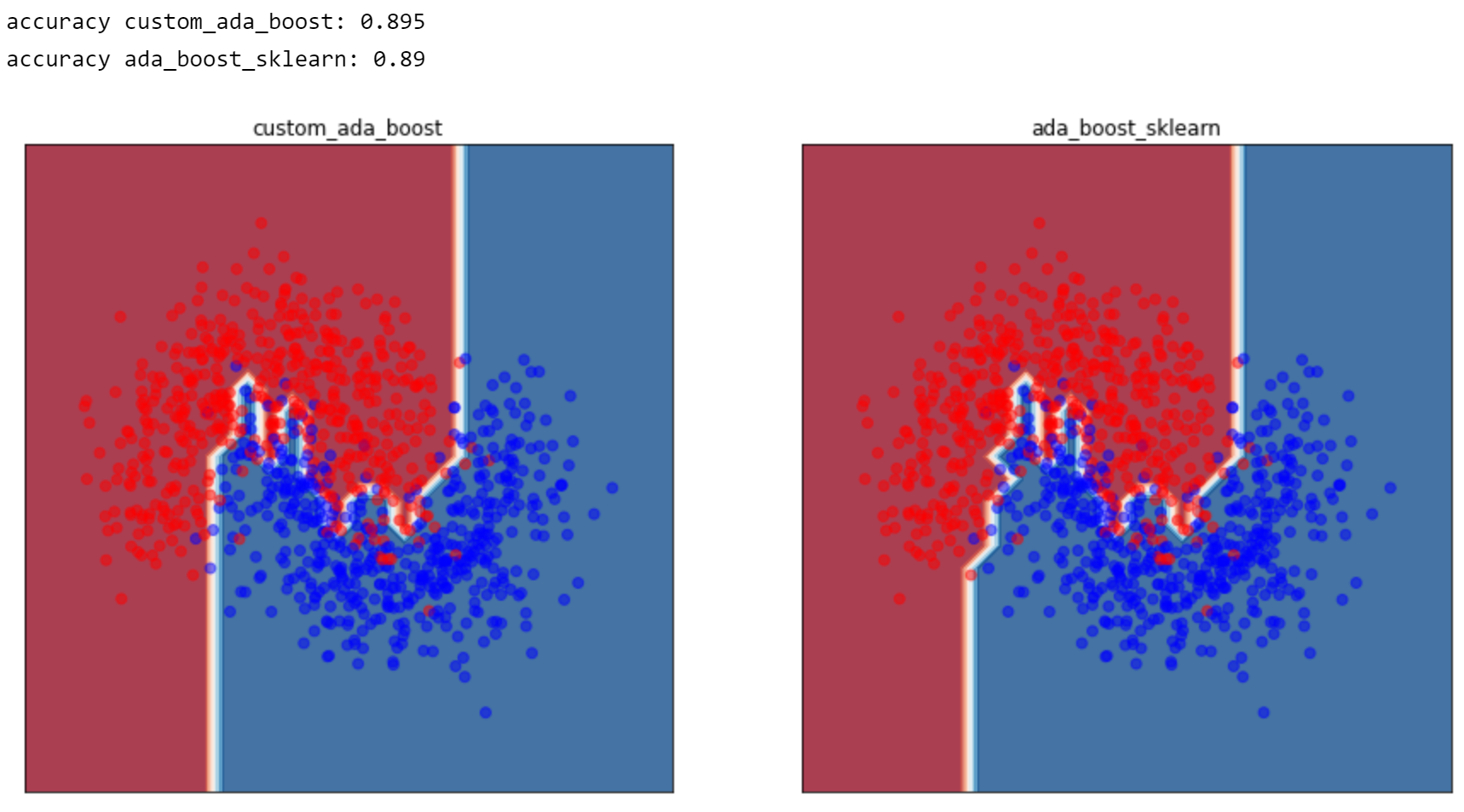
criteria

the decision boundary of the final implementation should look reasonably identical to the model from sklearn, and should achieve accuracy close to scikit :

$$|\text{your_accuracy} - \text{sklearn_accuracy}| \leq 0.005 \,.$$

Copy
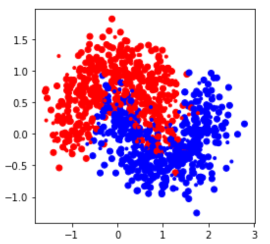
### Plot the dataset

X, y = make_moons(n_samples=1000, noise=0.3, random_state=0xC0FFEE)

# for convenience convert labels from {0, 1} to {-1, 1}
y[y == 0] = -1

Copy
X_train, X_test, y_train, y_test = train_test_split(X, y, test_size=0.2, random_state=0xC0FFEE)

x_min, x_max = X[:, 0].min() - .5, X[:, 0].max() + .5
y_min, y_max = X[:, 1].min() - .5, X[:, 1].max() + .5
xx, yy = np.meshgrid(np.linspace(x_min, x_max, 30),
                     np.linspace(y_min, y_max, 30))

cm = plt.cm.RdBu
cm_bright = ListedColormap(['#FF0000', '#0000FF'])

Copy
# Plot the training points
plt.figure(figsize=(4, 4))
plt.scatter(X_train[:, 0], X_train[:, 1], c=y_train, cmap=cm_bright)
plt.scatter(X_test[:, 0], X_test[:, 1], marker='.', c=y_test, cmap=cm_bright)
plt.show()

Copy
from sklearn.tree import DecisionTreeClassifier # base classifier

Now let us define functions to calculate alphas and distributions for AdaBoost algorithm

Copy

def ada_boost_alpha(y, y_pred_t, distribution):
    """
    Function, which calculates the weights of the linear combination of the classifiers.
    
    y_pred_t is a prediction of the t-th base classifier
    """
    distribution = (y!= y_pred_t) * distribution
    eps_t = np.sum(distribution)
    alpha = 0.5 * np.log((1-eps_t) / (eps_t))

    return alpha

def ada_boost_distribution(y, y_pred_t, distribution, alpha_t):
    """
    Function, which calculates sample weights
    
    y_pred_t is a prediction of the t-th base classifier
    """
    distribution = [w_i*np.exp(-alpha_t*y_i*y_pred_t_i) for w_i,y_i,y_pred_t_i in zip(distribution,y,y_pred_t)]    
    norm_term = np.sum(distribution)
    distribution = distribution/norm_term

    return distribution

Implement your own AdaBoost algorithm. Then compare it with the sklearn implementation.

Copy
class Boosting():
    """
    Generic class for construction of boosting models
    
    :param n_estimators: int, number of estimators (number of boosting rounds)
    :param base_classifier: callable, a function that creates a weak estimator. Weak estimator should support sample_weight argument
    :param get_alpha: callable, a function, that calculates new alpha given current distribution, prediction of the t-th base estimator,
                      boosting prediction at step (t-1) and actual labels
    :param get_distribution: callable, a function, that calculates samples weights given current distribution, prediction, alphas and actual labels
    """
    def __init__(self, n_estimators=50, base_classifier=None,
                 get_alpha=ada_boost_alpha, update_distribution=ada_boost_distribution):
        self.n_estimators = n_estimators # 弱学习器数量
        self.base_classifier = base_classifier # 弱学习器，传参DecisionTreeClassifier
        self.get_alpha = get_alpha # 弱分类器权重
        self.update_distribution = update_distribution # 更新权值分布
    # 进行拟合   
    def fit(self, X, y):
        n_samples = len(X) 
        distribution = np.ones(n_samples, dtype=float) / n_samples # 初始权值分布
        self.classifiers = [] 
        self.alphas = []
        # 循环所有样本特征
        for i in range(self.n_estimators):
            # create a new classifier 用特定的权值拟合一个分类器
            self.classifiers.append(self.base_classifier()) # 将当前层添加到索引中
            self.classifiers[-1].fit(X, y, sample_weight=distribution) # 训练弱学习器

            ### BEGIN Solution (do not delete this comment)
            

            # make a prediction 调用弱分类器进行预测
            y_pred_t = self.classifiers[-1].predict(X) 
            #update alphas, append new alpha to self.alphas 更新alpha
            self.alphas.append(self.get_alpha(y,y_pred_t,distribution))# 更新弱分类器权值
            
            # update distribution and normalize 更新权值 && 归一化
            distribution = self.update_distribution(y,y_pred_t,distribution,self.alphas[-1])/np.sum(distribution) # 更新弱分类器权值
            ### END Solution (do not delete this comment)

    
    def predict(self, X):
        final_predictions = np.zeros(X.shape[0]) # 预测结果初始化
    
        ### BEGIN Solution (do not delete this comment)
        
        #get the weighted votes of the classifiers
        for j in range(self.n_estimators):
            final_predictions += self.alphas[j]*self.classifiers[j].predict(X)
        final_predictions[final_predictions < 0] = -1
        final_predictions[final_predictions >= 0] = 1
        out = final_predictions 
        ### END Solution (do not delete this comment)

        return out

Copy
max_depth = 5
n_estimators = 100

get_base_clf = lambda: DecisionTreeClassifier(max_depth=max_depth)

### BEGIN Solution (do not delete this comment)

custom_ada_boost = Boosting(n_estimators=n_estimators,
                     base_classifier=get_base_clf)

ada_boost_sklearn = AdaBoostClassifier(DecisionTreeClassifier(max_depth=max_depth),
                                       algorithm="SAMME",
                                       n_estimators=n_estimators)

### END Solution (do not delete this comment)

Copy
custom_ada_boost.fit(X_train, y_train)
ada_boost_sklearn.fit(X_train, y_train)

Copy
classifiers = [custom_ada_boost, ada_boost_sklearn]
names = ['custom_ada_boost', 'ada_boost_sklearn']

Copy
# # test ensemble classifier
plt.figure(figsize=(15, 7))
for i, clf in enumerate(classifiers):
    prediction = clf.predict(X_test)

    # Put the result into a color plot
    ax = plt.subplot(1, len(classifiers), i + 1)
    Z = clf.predict(np.c_[xx.ravel(), yy.ravel()])
    Z = Z.reshape(xx.shape)
    ax.contourf(xx, yy, Z, cmap=cm, alpha=.8)

    # Plot also the training points
    ax.scatter(X[:, 0], X[:, 1], c=y, cmap=cm_bright, alpha=0.5)

    ax.set_xlim(xx.min(), xx.max())
    ax.set_ylim(yy.min(), yy.max())
    ax.set_xticks(())
    ax.set_yticks(())
    ax.set_title(names[i])

    print('accuracy {}: {}'.format(names[i], (prediction == y_test).sum() * 1. / len(y_test)))

结果如下