算法模型②
F检验:提出原假设和备择假设 之后计算统计量与理论值 最后比较
    F检验主要检验的是模型是否合理
 #即 正向验证与反向验证
主要是用来检验模型是否合理
# 导⼊第三⽅模块
import numpy as np
# 计算建模数据中因变量的均值
ybar=train.Profit.mean()
# 统计变量个数和观测个数
p=model2.df_model
n=train.shape[0]
# 计算回归离差平⽅和
RSS=np.sum((model2.fittedvalues-ybar)**2)
# 计算误差平⽅和
ESS=np.sum(model2.resid**2)
# 计算F统计量的值
F=(RSS/p)/(ESS/(n-p-1))
print('F统计量的值:',F)
F统计量的值:174.6372
t检验:
更加侧重于检验模型参数是否合理
#model.summary() # 绝对值越小影响越大
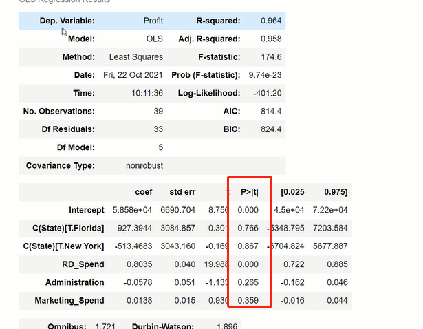
# 值越小 影响程度越大
线性回归模型短板与不足:
1、自变量个数大于样本量。
2、自变量直接存在多重共线性(值高度相关)。
为了解决上述问题 引入了 岭回归模型和lasso回归模型
岭回归模型:
在线性回归模型的基础之上添加一个l2惩罚项(平方项、正则项)
该模型最终转变成求解圆柱体与椭圆抛物线的焦点问题

公式呈现:
线性回归模型:J(β)=∑(y−Xβ)^2
岭回归模型:J(β)=∑(y−Xβ)^2+∑λβ^2
岭回归交叉验证参数:
RidgeCV(alphas=(0.1, 1.0, 10.0), fit_intercept=True, normalize=False,
scoring=None, cv=None)
# 参数
alphas:⽤于指定多个lambda值的元组或数组对象,默认该参数包含0.1、1和10三种值。
fit_intercept:bool类型参数,是否需要拟合截距项,默认为True。
normalize:bool类型参数,建模时是否需要对数据集做标准化处理,默认为False。
scoring:指定⽤于评估模型的度量⽅法。
cv:指定交叉验证的重数。
案例:
'''求最准确的Lamda值''' # 导入模块 from sklearn.linear_model import Ridge,RidgeCV # 读取糖尿病数据集 diabetes = pd.read_excel(r'diabetes.xlsx') # 构造自变量(剔除患者性别、年龄和因变量) predictors = diabetes.columns[2:-1] # 将数据集拆分为训练集和测试集 X_train, X_test, y_train, y_test = model_selection.train_test_split(diabetes[predictors], diabetes['Y'],test_size = 0.2, random_state = 1234) # 构造不同的Lamda值 Lambdas=np.logspace(-5,2,200) # 设置交叉验证的参数,对于每一个Lambda值,都执行10重交叉验证 ridge_cv = RidgeCV(alphas = Lambdas, normalize=True, scoring='neg_mean_squared_error', cv = 10) # 模型拟合 ridge_cv.fit(X_train, y_train) # 返回最佳的lambda值 ridge_best_Lambda = ridge_cv.alpha_ ridge_best_Lambda # 0.014649713983072863 '''基于最准确的Lamda值建模''' # 导入第三方包中的函数 from sklearn.metrics import mean_squared_error # 基于最佳的Lambda值建模 ridge = Ridge(alpha = ridge_best_Lambda, normalize=True) ridge.fit(X_train, y_train) # 返回岭回归系数 pd.Series(index = ['Intercept'] + X_train.columns.tolist(),data = [ridge.intercept_] + ridge.coef_.tolist()) # 预测 ridge_predict = ridge.predict(X_test) # 预测效果验证:均方根误差 RMSE = np.sqrt(mean_squared_error(y_test,ridge_predict)) RMSE # 53.119117887535204
Lasso回归模型:
在线性回归模型的基础之上添加一个l1惩罚项(绝对值项、正则项)
该模型最终转变成求解正方体与椭圆抛物线的焦点问题

Lasso回归交叉验证的参数:
LassoCV(alphas=None, fit_intercept=True,
normalize=False,max_iter=1000, tol=0.0001)
# 参数
alphas:指定具体的Lambda值列表⽤于模型的运算
fit_intercept:bool类型参数,是否需要拟合截距项,默认为True
normalize:bool类型参数,建模时是否需要对数据集做标准化处理,默认为False
max_iter:指定模型最⼤的迭代次数,默认为1000次
案例:
'''求最准确的Lamda值''' # 导入第三方模块中的函数 from sklearn.linear_model import Lasso,LassoCV # LASSO回归模型的交叉验证 lasso_cv = LassoCV(alphas = Lambdas, normalize=True, cv = 10, max_iter=10000) lasso_cv.fit(X_train, y_train) # 输出最佳的lambda值 lasso_best_alpha = lasso_cv.alpha_ lasso_best_alpha # 0.06294988990221888 '''基于最准确的Lamda值建模''' # 基于最佳的lambda值建模 lasso = Lasso(alpha = lasso_best_alpha, normalize=True, max_iter=10000) lasso.fit(X_train, y_train) # 返回LASSO回归的系数 xs=pd.Series(index = ['Intercept'] + X_train.columns.tolist(),data = [lasso.intercept_] + lasso.coef_.tolist()) xs # 预测 lasso_predict = lasso.predict(X_test) # 预测效果验证 RMSE = np.sqrt(mean_squared_error(y_test,lasso_predict)) RMSE # 53.06143725822573
思考:
岭回归和lasso回归的区别在哪?
#都是为了解决线性回归模型的短板 , 其区别在于 岭回归添加的惩罚项是平方值, lasso回归添加的惩罚项是绝对值 ,lasso回归相较于岭回归会更加简单
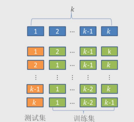
交叉验证:
1.将数据集拆分成k个样本量相当的数据组,组建无重叠样本。
2.从k组数据中挑选k-1组用于构建模型,剩下一组用于测试。
3.以此类推,获得k种训练集和测试集,每一个数据组都将参与构建以及测试。
4.从中选择准确度最高的模型
Logistic回归模型

# 将线性回归模型的公式做Logit变换即为Logistic回归模型
 将预测问题变成了0到1之间的概率问题
本质:

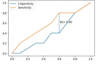
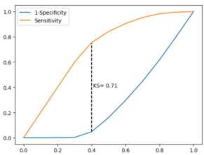
自定义绘制ks曲线的函数


# 导入第三方模块 import pandas as pd import numpy as np import matplotlib.pyplot as plt from sklearn import model_selection from sklearn import linear_model # 自定义绘制ks曲线的函数 def plot_ks(y_test, y_score, positive_flag): # 对y_test重新设置索引 y_test.index = np.arange(len(y_test)) # 构建目标数据集 target_data = pd.DataFrame({'y_test':y_test, 'y_score':y_score}) # 按y_score降序排列 target_data.sort_values(by = 'y_score', ascending = False, inplace = True) # 自定义分位点 cuts = np.arange(0.1,1,0.1) # 计算各分位点对应的Score值 index = len(target_data.y_score)*cuts scores = np.array(target_data.y_score)[index.astype('int')] # 根据不同的Score值,计算Sensitivity和Specificity Sensitivity = [] Specificity = [] for score in scores: # 正例覆盖样本数量与实际正例样本量 positive_recall = target_data.loc[(target_data.y_test == positive_flag) & (target_data.y_score>score),:].shape[0] positive = sum(target_data.y_test == positive_flag) # 负例覆盖样本数量与实际负例样本量 negative_recall = target_data.loc[(target_data.y_test != positive_flag) & (target_data.y_score<=score),:].shape[0] negative = sum(target_data.y_test != positive_flag) Sensitivity.append(positive_recall/positive) Specificity.append(negative_recall/negative) # 构建绘图数据 plot_data = pd.DataFrame({'cuts':cuts,'y1':1-np.array(Specificity),'y2':np.array(Sensitivity), 'ks':np.array(Sensitivity)-(1-np.array(Specificity))}) # 寻找Sensitivity和1-Specificity之差的最大值索引 max_ks_index = np.argmax(plot_data.ks) plt.plot([0]+cuts.tolist()+[1], [0]+plot_data.y1.tolist()+[1], label = '1-Specificity') plt.plot([0]+cuts.tolist()+[1], [0]+plot_data.y2.tolist()+[1], label = 'Sensitivity') # 添加参考线 plt.vlines(plot_data.cuts[max_ks_index], ymin = plot_data.y1[max_ks_index], ymax = plot_data.y2[max_ks_index], linestyles = '--') # 添加文本信息 plt.text(x = plot_data.cuts[max_ks_index]+0.01, y = plot_data.y1[max_ks_index]+plot_data.ks[max_ks_index]/2, s = 'KS= %.2f' %plot_data.ks[max_ks_index]) # 显示图例 plt.legend() # 显示图形 plt.show()
回归参数:
LogisticRegression(tol=0.0001, fit_intercept=True,class_weight=None, max_iter=100)
# 参数
tol:⽤于指定模型跌倒收敛的阈值
fit_intercept:bool类型参数,是否拟合模型的截距项,默认为True
class_weight:⽤于指定因变量类别的权重,如果为字典,则通过字典的形式{class_label:weight}传递每个类别的权重;如果为字符串'balanced',则每个分类的权重与实际样本中的⽐例成反⽐,当各分类存在严重不平衡时,设置为'balanced'会⽐较好;如果为None,则表示每个分类的权重相等
max_iter:指定模型求解过程中的最⼤迭代次数, 默认为100
案例1:
# 导入虚拟数据
virtual_data = pd.read_excel(r'virtual_data.xlsx')
# 应用自定义函数绘制k-s曲线
plot_ks(y_test = virtual_data.Class, y_score = virtual_data.Score,positive_flag = 'P')
案例2:求解模型参数
# 读取数据 sports = pd.read_csv(r'Run or Walk.csv') # 提取出所有自变量名称 predictors = sports.columns[4:] # 构建自变量矩阵 X = sports.ix[:,predictors] # 提取y变量值 y = sports.activity # 将数据集拆分为训练集和测试集 X_train, X_test, y_train, y_test = model_selection.train_test_split(X, y, test_size = 0.25, random_state = 1234) # 利用训练集建模 sklearn_logistic = linear_model.LogisticRegression() sklearn_logistic.fit(X_train, y_train) # 返回模型的各个参数 print(sklearn_logistic.intercept_, sklearn_logistic.coef_)
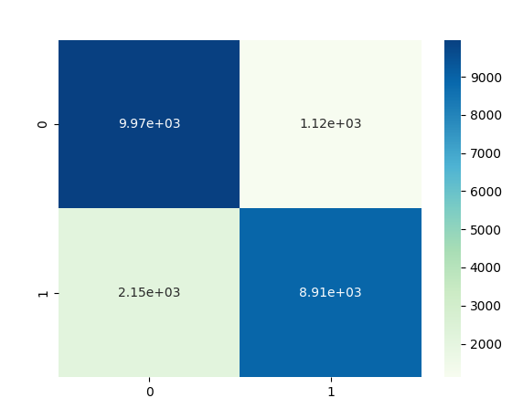
混淆矩阵:
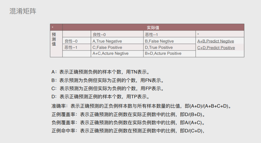
混淆矩阵的可视化(热力图)
# 混淆矩阵的可视化
# 导入第三方模块
import seaborn as sns
import matplotlib.pyplot as plt
%matplotlib
# 绘制热力图
sns.heatmap(cm, annot = True, fmt = '.2e',cmap = 'GnBu')
# 图形显示
plt.show()
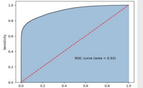
ROC曲线—面积图
通过计算AUC阴影部分的面积来判断模型是否合理(通常大于0.8表示基本准确)
# y得分为模型预测正例的概率 y_score = sklearn_logistic.predict_proba(X_test)[:,1] # 计算不同阈值下,fpr和tpr的组合值,其中fpr表示1-Specificity,tpr表示Sensitivity fpr,tpr,threshold = metrics.roc_curve(y_test, y_score) # 计算AUC的值 roc_auc = metrics.auc(fpr,tpr) # 绘制面积图 plt.stackplot(fpr, tpr, color='steelblue', alpha = 0.5, edgecolor = 'black') # 添加边际线 plt.plot(fpr, tpr, color='black', lw = 1) # 添加对角线 plt.plot([0,1],[0,1], color = 'red', linestyle = '--') # 添加文本信息 plt.text(0.5,0.3,'ROC curve (area = %0.2f)' % roc_auc) # 添加x轴与y轴标签 plt.xlabel('1-Specificity') plt.ylabel('Sensitivity') # 显示图形 plt.show()
# 调⽤⾃定义函数,绘制K-S曲线
plot_ks(y_test = y_test, y_score = y_score, positive_flag = 1)
求解流程:
# -----------------------第一步 建模 ----------------------- # # 导入第三方模块 import statsmodels.api as sm # 将数据集拆分为训练集和测试集 X_train, X_test, y_train, y_test = model_selection.train_test_split(X, y, test_size = 0.25, random_state = 1234) # 为训练集和测试集的X矩阵添加常数列1 X_train2 = sm.add_constant(X_train) X_test2 = sm.add_constant(X_test) # 拟合Logistic模型 sm_logistic = sm.Logit(y_train, X_train2).fit() # 返回模型的参数 sm_logistic.params # -----------------------第二步 预测构建混淆矩阵 ----------------------- # # 模型在测试集上的预测 sm_y_probability = sm_logistic.predict(X_test2) # 根据概率值,将观测进行分类,以0.5作为阈值 sm_pred_y = np.where(sm_y_probability >= 0.5, 1, 0) # 混淆矩阵 cm = metrics.confusion_matrix(y_test, sm_pred_y, labels = [0,1]) cm # -----------------------第三步 绘制ROC曲线 ----------------------- # # 计算真正率和假正率 fpr,tpr,threshold = metrics.roc_curve(y_test, sm_y_probability) # 计算auc的值 roc_auc = metrics.auc(fpr,tpr) # 绘制面积图 plt.stackplot(fpr, tpr, color='steelblue', alpha = 0.5, edgecolor = 'black') # 添加边际线 plt.plot(fpr, tpr, color='black', lw = 1) # 添加对角线 plt.plot([0,1],[0,1], color = 'red', linestyle = '--') # 添加文本信息 plt.text(0.5,0.3,'ROC curve (area = %0.2f)' % roc_auc) # 添加x轴与y轴标签 plt.xlabel('1-Specificity') plt.ylabel('Sensitivity') # 显示图形 plt.show() # -----------------------第四步 绘制K-S曲线 ----------------------- # # 调用自定义函数,绘制K-S曲线 sm_y_probability.index = np.arange(len(sm_y_probability)) plot_ks(y_test = y_test, y_score = sm_y_probability, positive_flag = 1) """ 模型评估方法 """ 1.ROC曲线:通过计算AUC阴影部分的面积来判断模型是否合理(通常大于0.8表示OK) 2.KS曲线:通过计算两条折现之间最大距离来衡量模型是否合理(通常大于0.4表示OK)
决策树与随机森林:
用于解决分类的问题,买不买走不走 吃不吃,通过预测问题来解决具体数值
这里的树其实是计算机底层的一种数据结构,与现实不同,可理解为自上而下生长
# 决策树
算法模型的概念,由三部分组成
根节点:树的起点
枝节点:即中间节点,和根节点一样也是条件判断
叶子节点:分支的终点

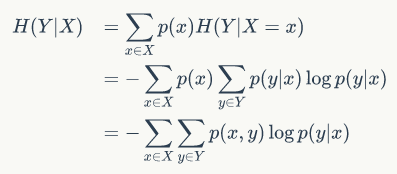
信息熵:
熵原本是物理学中的概念表示混乱程度在it领域表示信息量的大小

案例:

条件熵:
条件熵是信息熵的延伸,添加特定的条件后对信息熵进行分类
信息增益:
信息增益可以反映出某个条件是否对最终的分类有决定性的影响
在构建决策树时根节点与枝节点所放的条件按照信息增益由大到小排列

信息增益率:
信息增益会偏向取值较多的字段,为了避免这类情况的发生,提引进了信息增益率的概念,就是在计算信息增益时添加的惩罚项。

基尼指数:

基尼指数增益
自变量对应变量的影响程度

决策树参数模型说明:
DecisionTreeClassifier(criterion='gini', splitter='best',
max_depth=None,min_samples_split=2,
min_samples_leaf=1,max_leaf_nodes=None,
class_weight=None)
criterion:⽤于指定选择节点字段的评价指标,对于分类决策树,默认为'gini',表示采⽤基尼指数选
择节点的最佳分割字段;对于回归决策树,默认为'mse',表示使⽤均⽅误差选择节点的最佳分割字段
splitter:⽤于指定节点中的分割点选择⽅法,默认为'best',表示从所有的分割点中选择最佳分割点;
如果指定为'random',则表示随机选择分割点
max_depth:⽤于指定决策树的最⼤深度,默认为None,表示树的⽣⻓过程中对深度不做任何限制
min_samples_split:⽤于指定根节点或中间节点能够继续分割的最⼩样本量, 默认为2
min_samples_leaf:⽤于指定叶节点的最⼩样本量,默认为1
决策树案例:
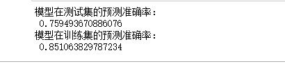
# 导入第三方模块 import pandas as pd import numpy as np import matplotlib.pyplot as plt from sklearn import model_selection from sklearn import linear_model # 读⼊数据 Titanic = pd.read_csv(r'Titanic.csv') Titanic # 删除⽆意义的变量,并检查剩余变量是否含有缺失值 Titanic.drop(['PassengerId','Name','Ticket','Cabin'], axis = 1, inplace = True) Titanic.isnull().sum(axis = 0) # 对Sex分组,⽤各组乘客的平均年龄填充各组中的缺失年龄 fillna_Titanic = [] for i in Titanic.Sex.unique(): update = Titanic.loc[Titanic.Sex == i,].fillna(value = {'Age': Titanic.Age[Titanic.Sex == i].mean()}, inplace = False) fillna_Titanic.append(update) Titanic = pd.concat(fillna_Titanic) # 使⽤Embarked变量的众数填充缺失值 Titanic.fillna(value = {'Embarked':Titanic.Embarked.mode()[0]}, inplace=True) # 将数值型的Pclass转换为类别型,否则⽆法对其哑变量处理 Titanic.Pclass = Titanic.Pclass.astype('category') # 哑变量处理 dummy = pd.get_dummies(Titanic[['Sex','Embarked','Pclass']]) # ⽔平合并Titanic数据集和哑变量的数据集 Titanic = pd.concat([Titanic,dummy], axis = 1) # 删除原始的Sex、Embarked和Pclass变量 Titanic.drop(['Sex','Embarked','Pclass'], inplace=True, axis = 1) # 取出所有⾃变量名称 predictors = Titanic.columns[1:] # 将数据集拆分为训练集和测试集,且测试集的⽐例为25% X_train, X_test, y_train, y_test = model_selection.train_test_split(Titanic[predictors], Titanic.Survived, test_size = 0.25, random_state = 1234) from sklearn.model_selection import GridSearchCV from sklearn import tree,metrics # 预设各参数的不同选项值 max_depth = [2,3,4,5,6] min_samples_split = [2,4,6,8] min_samples_leaf = [2,4,8,10,12] # 将各参数值以字典形式组织起来 parameters = {'max_depth':max_depth, 'min_samples_split':min_samples_split, 'min_samples_leaf':min_samples_leaf} # ⽹格搜索法,测试不同的参数值 grid_dtcateg = GridSearchCV(estimator = tree.DecisionTreeClassifier(), param_grid = parameters, cv=10) # 模型拟合 grid_dtcateg.fit(X_train, y_train) # 返回最佳组合的参数值 grid_dtcateg.param_grid # 构建分类决策树 CART_Class = tree.DecisionTreeClassifier(max_depth=3,min_samples_leaf=4,min_samples_split=2) # 模型拟合 decision_tree = CART_Class.fit(X_train,y_train) # 模型在测试集上的预测 pred = CART_Class.predict(X_test) # 模型的准确率 print('模型在测试集的预测准确率:\n',metrics.accuracy_score(y_test,pred)) print('模型在训练集的预测准确率:\n',metrics.accuracy_score(y_train,CART_Class.predict(X_train)))
随机森林:
随机森林中每颗决策树都不限制节点字段选择,
有多棵树组成的随机森林
在解决分类问题的时候采用投票法、解决预测问题的时候采用均值法

函数说明:
RandomForestClassifier(n_estimators=10, criterion='gini', max_depth=None,
min_samples_split=2, min_samples_leaf=1,
max_leaf_nodes=None, bootstrap=True, class_weight=None)
n_estimators:⽤于指定随机森林所包含的决策树个数
criterion:⽤于指定每棵决策树节点的分割字段所使⽤的度量标准,⽤于分类的随机森林,默认的
criterion值为'gini';⽤于回归的随机森林,默认的criterion值为'mse'
max_depth:⽤于指定每棵决策树的最⼤深度,默认不限制树的⽣⻓深度
min_samples_split:⽤于指定每棵决策树根节点或中间节点能够继续分割的最⼩样本量, 默认为2
k近邻模型
思想:
本质就是寻找x个样本,基于最近样本做预测
x不能过拟合(精度过高)也不能欠拟合(精度过低)

取值思路1:
取值思路2:

距离:
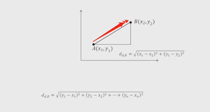
欧式距离:(两点之间直线距离)
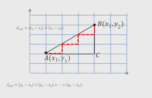
曼哈顿距离:(两点之间绕过障碍物的距离)
余弦相似度:(测量两个向量的夹角的余弦值来度量它们之间的相似性)
可以用于论文查重。

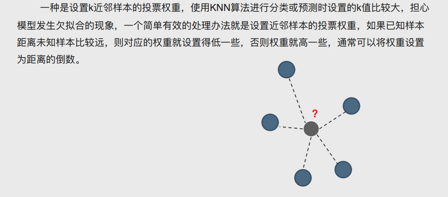
knn模型参数说明
neighbors.KNeighborsClassifier(n_neighbors=5, weights='uniform',p=2, metric='minkowski',)
# 参数
n_neighbors:⽤于指定近邻样本个数K,默认为5
weights:⽤于指定近邻样本的投票权重,默认为'uniform',表示所有近邻样本的投票权重⼀样;如果
为'distance',则表示投票权重与距离成反⽐,即近邻样本与未知类别的样本点距离越远,权重越⼩,
反之,权重越⼤
metric:⽤于指定距离的度量指标,默认为闵可夫斯基距离
p:当参数metric为闵可夫斯基距离时,p=1,表示计算点之间的曼哈顿距离;p=2,表示计算点之间的欧⽒距离,默认值为2