7. PyTorch可视化网络结构
7.1 可视化网络结构
7.1.1 使用torchinfo可视化网络结构
-
torchinfo的安装
# 安装方法一
pip install torchinfo
# 安装方法二
conda install -c conda-forge torchinfo
-
torchinfo的使用 -- totchinfo.summary(model, input_size[batch_size,channel,h,w])
import torchvision.models as models
from torchinfo import summary
resnet18 = models.resnet18() # 实例化模型
summary(resnet18, (1, 3, 224, 224)) # 1:batch_size 3:图片的通道数 224: 图片的高宽
-
torchinfo的结构化输出
=========================================================================================
Layer (type:depth-idx)                   Output Shape              Param #
=========================================================================================
ResNet                                   --                        --
├─Conv2d: 1-1                            [1, 64, 112, 112]         9,408
├─BatchNorm2d: 1-2                       [1, 64, 112, 112]         128
├─ReLU: 1-3                              [1, 64, 112, 112]         --
├─MaxPool2d: 1-4                         [1, 64, 56, 56]           --
├─Sequential: 1-5                        [1, 64, 56, 56]           --
│    └─BasicBlock: 2-1                   [1, 64, 56, 56]           --
│    │    └─Conv2d: 3-1                  [1, 64, 56, 56]           36,864
│    │    └─BatchNorm2d: 3-2             [1, 64, 56, 56]           128
│    │    └─ReLU: 3-3                    [1, 64, 56, 56]           --
│    │    └─Conv2d: 3-4                  [1, 64, 56, 56]           36,864
│    │    └─BatchNorm2d: 3-5             [1, 64, 56, 56]           128
│    │    └─ReLU: 3-6                    [1, 64, 56, 56]           --
│    └─BasicBlock: 2-2                   [1, 64, 56, 56]           --
│    │    └─Conv2d: 3-7                  [1, 64, 56, 56]           36,864
│    │    └─BatchNorm2d: 3-8             [1, 64, 56, 56]           128
│    │    └─ReLU: 3-9                    [1, 64, 56, 56]           --
│    │    └─Conv2d: 3-10                 [1, 64, 56, 56]           36,864
│    │    └─BatchNorm2d: 3-11            [1, 64, 56, 56]           128
│    │    └─ReLU: 3-12                   [1, 64, 56, 56]           --
├─Sequential: 1-6                        [1, 128, 28, 28]          --
│    └─BasicBlock: 2-3                   [1, 128, 28, 28]          --
│    │    └─Conv2d: 3-13                 [1, 128, 28, 28]          73,728
│    │    └─BatchNorm2d: 3-14            [1, 128, 28, 28]          256
│    │    └─ReLU: 3-15                   [1, 128, 28, 28]          --
│    │    └─Conv2d: 3-16                 [1, 128, 28, 28]          147,456
│    │    └─BatchNorm2d: 3-17            [1, 128, 28, 28]          256
│    │    └─Sequential: 3-18             [1, 128, 28, 28]          8,448
│    │    └─ReLU: 3-19                   [1, 128, 28, 28]          --
│    └─BasicBlock: 2-4                   [1, 128, 28, 28]          --
│    │    └─Conv2d: 3-20                 [1, 128, 28, 28]          147,456
│    │    └─BatchNorm2d: 3-21            [1, 128, 28, 28]          256
│    │    └─ReLU: 3-22                   [1, 128, 28, 28]          --
│    │    └─Conv2d: 3-23                 [1, 128, 28, 28]          147,456
│    │    └─BatchNorm2d: 3-24            [1, 128, 28, 28]          256
│    │    └─ReLU: 3-25                   [1, 128, 28, 28]          --
├─Sequential: 1-7                        [1, 256, 14, 14]          --
│    └─BasicBlock: 2-5                   [1, 256, 14, 14]          --
│    │    └─Conv2d: 3-26                 [1, 256, 14, 14]          294,912
│    │    └─BatchNorm2d: 3-27            [1, 256, 14, 14]          512
│    │    └─ReLU: 3-28                   [1, 256, 14, 14]          --
│    │    └─Conv2d: 3-29                 [1, 256, 14, 14]          589,824
│    │    └─BatchNorm2d: 3-30            [1, 256, 14, 14]          512
│    │    └─Sequential: 3-31             [1, 256, 14, 14]          33,280
│    │    └─ReLU: 3-32                   [1, 256, 14, 14]          --
│    └─BasicBlock: 2-6                   [1, 256, 14, 14]          --
│    │    └─Conv2d: 3-33                 [1, 256, 14, 14]          589,824
│    │    └─BatchNorm2d: 3-34            [1, 256, 14, 14]          512
│    │    └─ReLU: 3-35                   [1, 256, 14, 14]          --
│    │    └─Conv2d: 3-36                 [1, 256, 14, 14]          589,824
│    │    └─BatchNorm2d: 3-37            [1, 256, 14, 14]          512
│    │    └─ReLU: 3-38                   [1, 256, 14, 14]          --
├─Sequential: 1-8                        [1, 512, 7, 7]            --
│    └─BasicBlock: 2-7                   [1, 512, 7, 7]            --
│    │    └─Conv2d: 3-39                 [1, 512, 7, 7]            1,179,648
│    │    └─BatchNorm2d: 3-40            [1, 512, 7, 7]            1,024
│    │    └─ReLU: 3-41                   [1, 512, 7, 7]            --
│    │    └─Conv2d: 3-42                 [1, 512, 7, 7]            2,359,296
│    │    └─BatchNorm2d: 3-43            [1, 512, 7, 7]            1,024
│    │    └─Sequential: 3-44             [1, 512, 7, 7]            132,096
│    │    └─ReLU: 3-45                   [1, 512, 7, 7]            --
│    └─BasicBlock: 2-8                   [1, 512, 7, 7]            --
│    │    └─Conv2d: 3-46                 [1, 512, 7, 7]            2,359,296
│    │    └─BatchNorm2d: 3-47            [1, 512, 7, 7]            1,024
│    │    └─ReLU: 3-48                   [1, 512, 7, 7]            --
│    │    └─Conv2d: 3-49                 [1, 512, 7, 7]            2,359,296
│    │    └─BatchNorm2d: 3-50            [1, 512, 7, 7]            1,024
│    │    └─ReLU: 3-51                   [1, 512, 7, 7]            --
├─AdaptiveAvgPool2d: 1-9                 [1, 512, 1, 1]            --
├─Linear: 1-10                           [1, 1000]                 513,000
=========================================================================================
Total params: 11,689,512
Trainable params: 11,689,512
Non-trainable params: 0
Total mult-adds (G): 1.81
=========================================================================================
Input size (MB): 0.60
Forward/backward pass size (MB): 39.75
Params size (MB): 46.76
Estimated Total Size (MB): 87.11
=========================================================================================
注意:
当你使用的是colab或者jupyter notebook时,想要实现该方法,summary()一定是该单元(即notebook中的cell)的返回值,否则我们就需要使用print(summary(...))来可视化。
7.2 CNN可视化
首先加载模型,并确定模型的层信息:
import torch
from torchvision.models import vgg11

model = vgg11(pretrained=True)
## 可以通过调用nn.Module的named_children()方法来查看这个nn.Module的直接子级的模块:
print(dict(model.features.named_children()))

输出:
{'0': Conv2d(3, 64, kernel_size=(3, 3), stride=(1, 1), padding=(1, 1)),
 '1': ReLU(inplace=True),
 '2': MaxPool2d(kernel_size=2, stride=2, padding=0, dilation=1, ceil_mode=False),
 '3': Conv2d(64, 128, kernel_size=(3, 3), stride=(1, 1), padding=(1, 1)),
 '4': ReLU(inplace=True),
 '5': MaxPool2d(kernel_size=2, stride=2, padding=0, dilation=1, ceil_mode=False),
 '6': Conv2d(128, 256, kernel_size=(3, 3), stride=(1, 1), padding=(1, 1)),
 '7': ReLU(inplace=True),
 '8': Conv2d(256, 256, kernel_size=(3, 3), stride=(1, 1), padding=(1, 1)),
 '9': ReLU(inplace=True),
 '10': MaxPool2d(kernel_size=2, stride=2, padding=0, dilation=1, ceil_mode=False),
 '11': Conv2d(256, 512, kernel_size=(3, 3), stride=(1, 1), padding=(1, 1)),
 '12': ReLU(inplace=True),
 '13': Conv2d(512, 512, kernel_size=(3, 3), stride=(1, 1), padding=(1, 1)),
 '14': ReLU(inplace=True),
 '15': MaxPool2d(kernel_size=2, stride=2, padding=0, dilation=1, ceil_mode=False),
 '16': Conv2d(512, 512, kernel_size=(3, 3), stride=(1, 1), padding=(1, 1)),
 '17': ReLU(inplace=True),
 '18': Conv2d(512, 512, kernel_size=(3, 3), stride=(1, 1), padding=(1, 1)),
 '19': ReLU(inplace=True),
 '20': MaxPool2d(kernel_size=2, stride=2, padding=0, dilation=1, ceil_mode=False)}
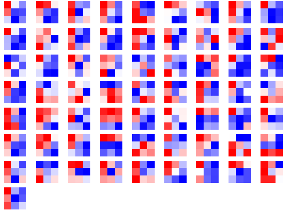
卷积核对应的应为卷积层(Conv2d),这里以第“3”层为例,可视化对应的参数:
conv1 = dict(model.features.named_children())['3']
kernel_set = conv1.weight.detach() # .detach(),使两个计算图的梯度传递断开,使目标从计算图中脱离出来。
num = len(conv1.weight.detach())
print(kernel_set.shape)
for i in range(0,num):
    i_kernel = kernel_set[i]
    plt.figure(figsize=(20, 17))
    if (len(i_kernel)) > 1:
        for idx, filer in enumerate(i_kernel):
            plt.subplot(9, 9, idx+1)
            plt.axis('off')
            plt.imshow(filer[ :, :].detach(),cmap='bwr')

输出:
torch.Size([128, 64, 3, 3])
由于第“3”层的特征图由64维变为128维,因此共有128*64个卷积核,其中部分卷积核可视化效果如下图所示:
7.2.2 CNN特征图可视化方法
定义:输入的原始图像经过每次卷积层得到的数据称为特征图。
目的:查看模型提取到的特征是什么样子的
在PyTorch中,提供了一个叫做hook的专用的接口使得网络在前向传播过程中能够获取到特征图。
class Hook(nn.Module):
    def __init__(self):
        self.module_name = []
        self.feature_in_hook = []
        self.feature_out_hook =[]

    def __call__(self, module, fea_in, fea_out):
        print("hooker working", self)
        self.module_name.append(module.__class__)
        self.feature_in_hook.append(fea_in)
        self.feature_out_hppk.append(fea_out)
        return None

def plot_feature(model, idx, inputs):
    hh = Hook()
    model.features[idx].register_forward_hook(hh)

    # forward_model(model,False)
    model.eval()
    _ = model(inputs)
    print(hh.module_name)
    print((hh.features_in_hook[0][0].shape))
    print((hh.features_out_hook[0].shape))

    out1 = hh.features_out_hook[0]

    total_ft  = out1.shape[1]
    first_item = out1[0].cpu().clone()

    plt.figure(figsize=(20, 17))

    for ftidx in range(total_ft):
        if ftidx > 99:
            break
        ft = first_item[ftidx]
        plt.subplot(10, 10, ftidx+1)

        plt.axis('off')
        #plt.imshow(ft[ :, :].detach(),cmap='gray')
        plt.imshow(ft[ :, :].detach())
首先实现了一个hook类,之后在plot_feature函数中,将该hook类的对象注册到要进行可视化的网络的某层中。
model在进行前向传播的时候会调用hook的__call__函数,也就是在那里存储了当前层的输入和输出。
这里的features_out_hook 是一个list,每次前向传播一次,都是调用一次,也就是features_out_hook 长度会增加1。
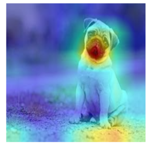
7.2.3 CNN class activation map可视化方法
class activation map (CAM)的作用是判断哪些变量对模型来说是重要的,在CNN可视化的场景下,即判断图像中哪些像素点对预测结果是重要的。
所需库:grad-cam库
例子:
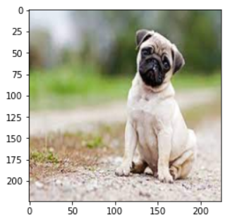
import torch
from torchvision.models import vgg11,resnet18,resnet101,resnext101_32x8d
import matplotlib.pyplot as plt
from PIL import Image
import numpy as np

model = vgg11(pretrained=True)
img_path = './dog.png'
# resize操作是为了和传入神经网络训练图片大小一致
img = Image.open(img_path).resize((224,224))
# 需要将原始图片转为np.float32格式并且在0-1之间
rgb_img = np.float32(img)/255
plt.imshow(img)
from pytorch_grad_cam import GradCAM,ScoreCAM,GradCAMPlusPlus,AblationCAM,XGradCAM,EigenCAM,FullGrad
from pytorch_grad_cam.utils.model_targets import ClassifierOutputTarget
from pytorch_grad_cam.utils.image import show_cam_on_image

target_layers = [model.features[-1]]
# 选取合适的类激活图,但是ScoreCAM和AblationCAM需要batch_size
cam = GradCAM(model=model,target_layers=target_layers)
targets = [ClassifierOutputTarget(preds)]
# 上方preds需要设定,比如ImageNet有1000类,这里可以设为200
grayscale_cam = cam(input_tensor=img_tensor, targets=targets)
grayscale_cam = grayscale_cam[0, :]
cam_img = show_cam_on_image(rgb_img, grayscale_cam, use_rgb=True)
print(type(cam_img))
Image.fromarray(cam_img)
7.2.4 使用FlashTorch快速实现CNN可视化
-
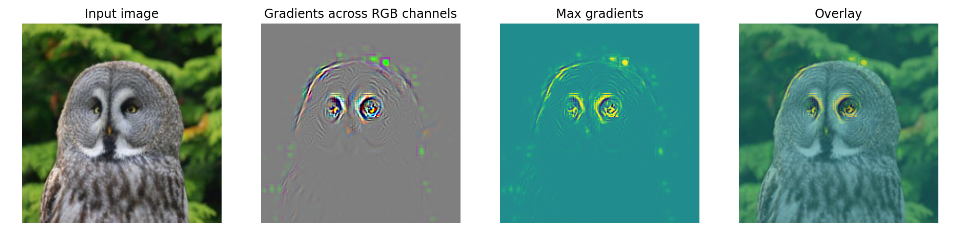
可视化梯度
import matplotlib.pyplot as plt
import torchvision.models as models
from flashtorch.utils import apply_transforms, load_image
from flashtorch.saliency import Backprop

model = models.alexnet(pretrained=True)
backprop = Backprop(model)

image = load_image('/content/images/great_grey_owl.jpg')
owl = apply_transforms(image)

target_class = 24
backprop.visualize(owl, target_class, guided=True, use_gpu=True)
-
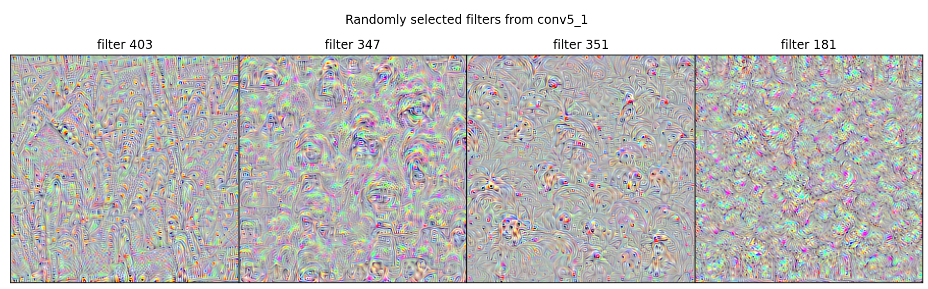
可视化卷积核
import torchvision.models as models
from flashtorch.activmax import GradientAscent

model = models.vgg16(pretrained=True)
g_ascent = GradientAscent(model.features)

# specify layer and filter info
conv5_1 = model.features[24]
conv5_1_filters = [45, 271, 363, 489]

g_ascent.visualize(conv5_1, conv5_1_filters, title="VGG16: conv5_1")
7.3 使用TensorBoard可视化训练过程
工具:tensorboardX 或 PyTorch自带的tensorboard
可以将TensorBoard看做一个记录员,它可以记录我们指定的数据,包括模型每一层的feature map,权重,以及训练loss等等。TensorBoard将记录下来的内容保存在一个用户指定的文件夹里,程序不断运行中TensorBoard会不断记录。记录下的内容可以通过网页的形式加以可视化。
7.3.1 TensorBoard的配置与启动
首先指定一个文件夹供TensorBoard保存记录下来的数据。
然后调用tensorboard中的SummaryWriter作为上述“记录员”
from tensorboardX import SummaryWriter

writer = SummaryWriter('./runs')
若使用PyTorch自带的tensorboard,则采用如下方式import:
from torch.utils.tensorboard import SummaryWriter
tensorboard异地可视化,在命令行中输入:
tensorboard --logdir=/path/to/logs/ --port=xxxx
其中“path/to/logs/"是指定的保存tensorboard记录结果的文件路径(等价于上面的“./runs",port是外部访问TensorBoard的端口号,可以通过访问ip:port访问tensorboard,这一操作和jupyter notebook的使用类似。如果不是在服务器远程使用的话则不需要配置port。
7.3.2 TensorBoard模型结构可视化
首先定义模型:
import torch.nn as nn

class Net(nn.Module):
    def __init__(self):
        super(Net, self).__init__()
        self.conv1 = nn.Conv2d(in_channels=3,out_channels=32,kernel_size = 3)
        self.pool = nn.MaxPool2d(kernel_size = 2,stride = 2)
        self.conv2 = nn.Conv2d(in_channels=32,out_channels=64,kernel_size = 5)
        self.adaptive_pool = nn.AdaptiveMaxPool2d((1,1))
        self.flatten = nn.Flatten()
        self.linear1 = nn.Linear(64,32)
        self.relu = nn.ReLU()
        self.linear2 = nn.Linear(32,1)
        self.sigmoid = nn.Sigmoid()

    def forward(self,x):
        x = self.conv1(x)
        x = self.pool(x)
        x = self.conv2(x)
        x = self.pool(x)
        x = self.adaptive_pool(x)
        x = self.flatten(x)
        x = self.linear1(x)
        x = self.relu(x)
        x = self.linear2(x)
        y = self.sigmoid(x)
        return y

model = Net()
print(model)

输出:
Net(
  (conv1): Conv2d(3, 32, kernel_size=(3, 3), stride=(1, 1))
  (pool): MaxPool2d(kernel_size=2, stride=2, padding=0, dilation=1, ceil_mode=False)
  (conv2): Conv2d(32, 64, kernel_size=(5, 5), stride=(1, 1))
  (adaptive_pool): AdaptiveMaxPool2d(output_size=(1, 1))
  (flatten): Flatten(start_dim=1, end_dim=-1)
  (linear1): Linear(in_features=64, out_features=32, bias=True)
  (relu): ReLU()
  (linear2): Linear(in_features=32, out_features=1, bias=True)
  (sigmoid): Sigmoid()
)
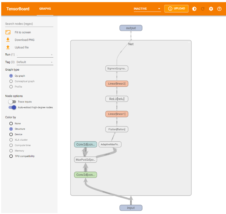
可视化模型的思路为:给定一个输入数据,前向传播后得到模型的结构,再通过TensorBoard进行可视化,使用add_graph:
writer.add_graph(model, input_to_model = torch.rand(1, 3, 224, 224))
writer.close()
7.3.3 TensorBoard图像可视化
-
对于单张图片的显示使用add_image
-
对于多张图片的显示使用add_images
-
有时需要使用torchvision.utils.make_grid将多张图片拼成一张图片后,用writer.add_image显示
# 仅查看一张图片
writer = SummaryWriter('./pytorch_tb')
writer.add_image('images[0]', images[0])
writer.close()

# 将多张图片拼接成一张图片,中间用黑色网格分割
# create grid of images
writer = SummaryWriter('./pytorch_tb')
img_grid = torchvision.utils.make_grid(images)
writer.add_image('image_grid', img_grid)
writer.close()

# 将多张图片直接写入
writer = SummaryWriter('./pytorch_tb')
writer.add_images("images",images,global_step = 0)
writer.close()
7.3.3 TensorBoard连续变量可视化
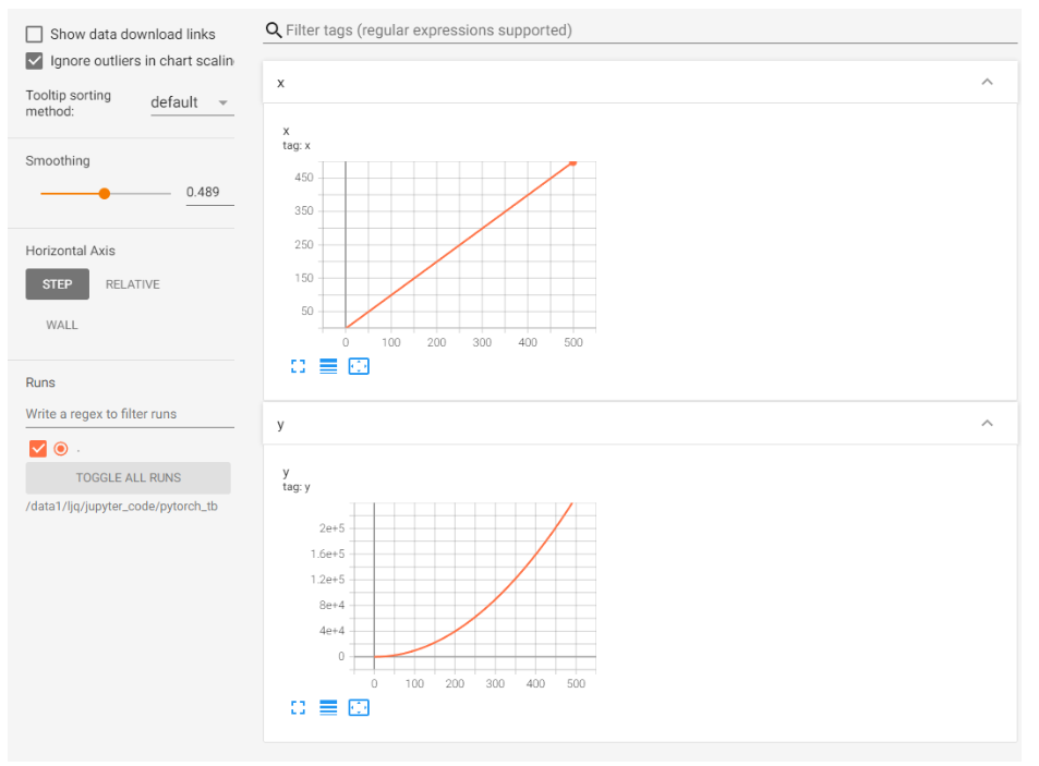
通过add_scalar实现:
writer = SummaryWriter('./pytorch_tb')
for i in range(500):
    x = i
    y = x**2
    writer.add_scalar("x", x, i) #日志中记录x在第step i 的值
    writer.add_scalar("y", y, i) #日志中记录y在第step i 的值
writer.close()
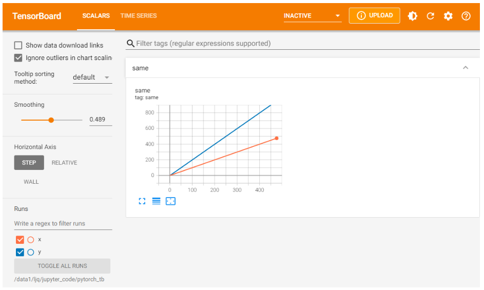
若想在同张图中显示多个曲线,则需要分别建立存放子路径(使用SummaryWriter指定路径即可自动创建,但需要在tensorboard运行目录下),同时在add_scalar中修改曲线的标签使其一致即可:
writer1 = SummaryWriter('./pytorch_tb/x')
writer2 = SummaryWriter('./pytorch_tb/y')
for i in range(500):
    x = i
    y = x*2
    writer1.add_scalar("same", x, i) #日志中记录x在第step i 的值
    writer2.add_scalar("same", y, i) #日志中记录y在第step i 的值
writer1.close()
writer2.close()
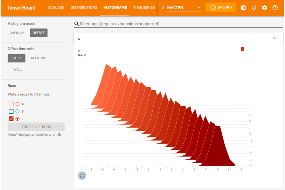
7.3.4 TensorBoard参数分布可视化
通过add_histogram实现:
import torch
import numpy as np

# 创建正态分布的张量模拟参数矩阵
def norm(mean, std):
    t = std * torch.randn((100, 20)) + mean
    return t

writer = SummaryWriter('./pytorch_tb/')
for step, mean in enumerate(range(-10, 10, 1)):
    w = norm(mean, 1)
    writer.add_histogram("w", w, step)
    writer.flush()
writer.close()

 浙公网安备 33010602011771号