基于matlab的史密斯圆图演示仿真图
1.算法描述
史密斯图表(Smith chart,又称史密斯圆图)是在反射系散平面上标绘有归一化输入阻抗(或导纳)等值圆族的计算图。是一款用于电机与电子工程学的图表,主要用于传输线的阻抗匹配上。该图由三个圆系构成,用以在传输线和某些波导问题中利用图解法求解,以避免繁琐的运算。一条传输线(transmission line)的电阻抗力(impedance)会随其长度而改变,要设计一套匹配(matching)的线路,需要通过不少繁复的计算程序,史密夫图表的特点便是省略一些计算程序。
史密斯图表的基本在于以下的算式:
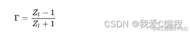
当中的Γ代表其线路的反射系数(reflection coefficient),即S参数(S-parameter)里的S11,ZL是归一负载值,即ZL / Z0。当中,ZL是线路本身的负载值,Z0是传输线的特征阻抗(本征阻抗)值,通常会使用50Ω。
图表中的圆形线代表电阻抗力的实数值,即电阻值,中间的横线与向上和向下散出的线则代表电阻抗力的虚数值,即由电容或电感在高频下所产生的阻力,当中向上的是正数,向下的是负数。图表最中间的点(1+j0)代表一个已匹配(matched)的电阻数值(ZL),同时其反射系数的值会是零。图表的边缘代表其反射系数的长度是1,即100%反射。在图边的数字代表反射系数的角度(0-180度)和波长(由零至半个波长)。
史密斯圆图: 反射系数圆图+阻抗/导纳圆图。输入阻抗不易直接测得,通过测量反射系数间接获得输入阻抗值。史密斯圆图中反射系数和输入阻抗一一对应。
史密斯圆图的应用:
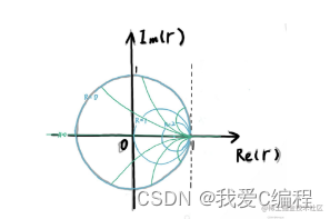
已知传输线的特性阻抗=50Ω,传输线的负载阻抗为=(50+j50)Ω,求离负载z=0.1λ处的等效阻抗。解:=/=1+j1 R=1 X=1
找到R=1的电阻圆和X=1的电抗圆的交点A,连接OA并延长交电长度刻度圆于B,OA顺时针旋转电长度0.1λ交电长度刻度圆于C,连接OC,交c1于P(据此读出|r|和Φ),过P点的R和X就是离负载z=0.1λ处的归一化输入阻抗。
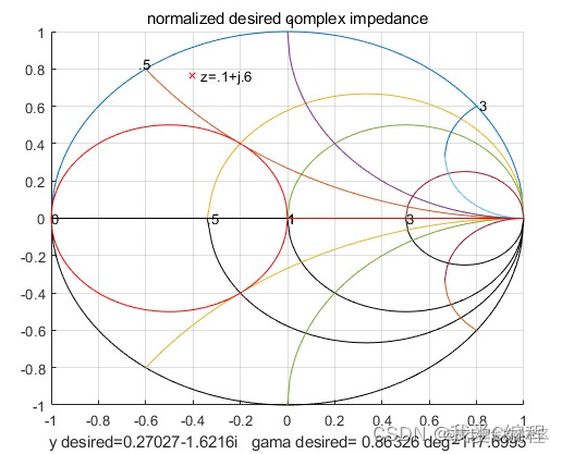
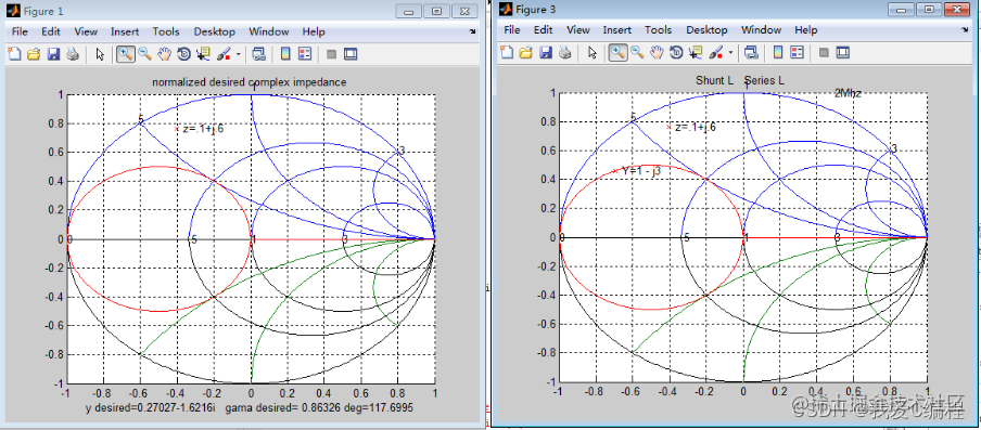
2.仿真效果预览
matlab2022a仿真结果如下:
3.MATLAB核心程序
if (deltaZP > 0 & imag(s)==0) % Shunt L Series C zInterceptP
	%case1
	shuntL=Zo/(s*w)
    seriesC=1/(w*abs(deltaZP*Zo))
	figure(2)
	smith3
	gama1=(zInterceptP-1)/(zInterceptP+1) %reflection coeffients of the interscetion to 1+js
	t=num2str(s);
	s4=[ '  Y=1 - j' t]
	plot(gama1,'rx')
	text(real(gama1),imag(gama1),s4) %plot intersection point
    s1=['Shunt L ' num2str(shuntL) '  Series C '  num2str(seriesC)] %list 2 element match on figure
	title(s1)
	plot(gama,'rx') %plot desired complex impedance
	text(real(gama),imag(gama),s3)
	text(.5,1,s5)
    %check solution
    [zTest]=shuntL_seriesC(shuntL,seriesC,w,Zo)
    xlabel(['actual impdeance=' num2str(zTest)])

    %*******************************************
elseif (deltaZP < 0 & imag(s)==0) % Shunt L Series L zInterceptP
	%case2
	shuntL=Zo/(w*s)
    seriesL=abs(deltaZP*Zo)/w
	figure(3)
	smith3
	gama1=(zInterceptP-1)/(zInterceptP+1)
	t=num2str(s);
	s4=[ '  Y=1 - j' t]
	plot(gama1,'rx')
	text(real(gama1),imag(gama1),s4)
    s1=['Shunt L ' num2str(shuntL) '  Series L '  num2str(seriesL)]
	title(s1)
	plot(gama,'rx')
	text(real(gama),imag(gama),s3)
	text(.5,1,s5)
    [zTest]=shuntL_seriesL(shuntL,seriesL,w,Zo)
    xlabel(['actual impdeance=' num2str(zTest)])
    %*******************************************
end

    if (deltaZM < 0 & imag(s)==0) % Shunt C Series L zInterceptM
	%case3
    shuntC=s/(Zo*w)
    seriesL=abs(deltaZM*Zo)/w
	figure(4)
	smith3
	gama1=(zInterceptM-1)/(zInterceptM+1)
	t=num2str(s);
	s4=[ '  Y=1 +  j' t]
	plot(gama1,'rx')
	text(real(gama1),imag(gama1),s4)
    s1=['Shunt C ' num2str(shuntC) '  Series L '  num2str(seriesL)]
	title(s1)
	plot(gama,'rx')
	text(real(gama),imag(gama),s3)
	text(.5,1,s5)
    [zTest]=shuntC_seriesL(shuntC,seriesL,w,Zo)
    xlabel(['actual impdeance=' num2str(zTest)])

    %*******************************************
elseif (deltaZM > 0 & imag(s)==0) % Shunt C Series C zInterceptM
	%case4
	shuntC=s/(Zo*w)
    seriesC=1/(Zo*deltaZM*w)
	figure(5)
	smith3
	gama1=(zInterceptM-1)/(zInterceptM+1)
	t=num2str(s);
	s4=[ '  Y=1 + j' t]
	plot(gama1,'rx')
	text(real(gama1),imag(gama1),s4)
    s1=['Shunt C ' num2str(shuntC) '  Series C '  num2str(seriesC)]
	title(s1)
	plot(gama,'rx')
	text(real(gama),imag(gama),s3)
	text(.5,1,s5)
    [zTest]=shuntC_seriesC(shuntC,seriesC,w,Zo)
    xlabel(['actual impdeance=' num2str(zTest)])

    %*******************************************
end

 浙公网安备 33010602011771号