m基于ESN+BP神经网络的数据预测算法matlab仿真,测试数据为太阳黑子变化数据
1.算法描述
在人工神经网络的发展历史上,感知机(Multilayer Perceptron,MLP)网络曾对人工神经网络的发展发挥了极大的作用,也被认为是一种真正能够使用的人工神经网络模型,它的出现曾掀起了人们研究人工神经元网络的热潮。单层感知网络(M-P模型)做为最初的神经网络,具有模型清晰、结构简单、计算量小等优点。但是,随着研究工作的深入,人们发现它还存在不足,例如无法处理非线性问题,即使计算单元的作用函数不用阀函数而用其他较复杂的非线性函数,仍然只能解决线性可分问题.不能实现某些基本功能,从而限制了它的应用。增强网络的分类和识别能力、解决非线性问题的唯一途径是采用多层前馈网络,即在输入层和输出层之间加上隐含层。构成多层前馈感知器网络。
BP神经网络具有任意复杂的模式分类能力和优良的多维函数映射能力,解决了简单感知器不能解决的异或(Exclusive OR,XOR)和一些其他问题。从结构上讲,BP网络具有输入层、隐藏层和输出层;从本质上讲,BP算法就是以网络误差平方为目标函数、采用梯度下降法来计算目标函数的最小值。
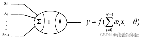
神经网络主要由处理单元、网络拓扑结构、训练规则组成。处理单元是神经网络的基本操作单元,用以模拟人脑神经元的功能。一个处理单元有多个输入、输出,输入端模拟脑神经的树突功能,起信息传递作用;输出端模拟脑神经的轴突功能,将处理后的信息传给下一个处理单元,如图1.1所示。
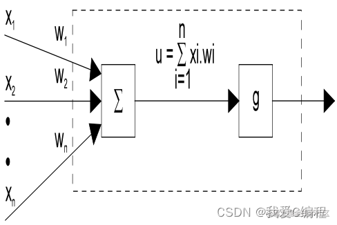
基本的神经处理单元其等效于人体的神经元,如图2所示,
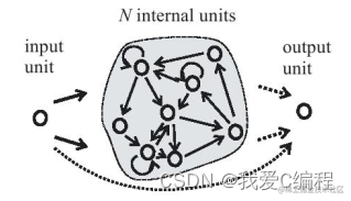
ESN是Jaeger于2001年提出一种新型递归神经网络,ESN一经提出便成为学术界的热点,并被大量地应用到各种不同的领域中,包括动态模式分类、机器人控制、对象跟踪核运动目标检测、事件监测等,尤其是在时间序列预测问题上,取得了较为突出的贡献。Jaeger本人在提出这种神经网络的第二年便在国际知名期刊上发表了关于将ESN网络用于时间序列预测的文章,为后来其发展做出了巨大的贡献。另外,国内大连理工大学的韩敏等人在ESN的使用方面也做出了突出的贡献。
ESN具有以下特点:
大且稀疏生物连接,RNN被当做一个动态水库
动态水库可以由输入或/和输出的反馈激活
水库的连接权值不会被训练改变?
只有水库的输出单元的权值随训练改变,因此训练是一个线性回归任务
假设有ESN是一个可调谐的sin波生成器:
黑色箭头是指固定的输入和反馈连接
红色箭头指可训练的输出连接
灰色表示循环内连接的动态水库
在原始的ESN中,权值的计算是通过pseudoinverse.m这个函数进行计算的,其内容就是:

即:

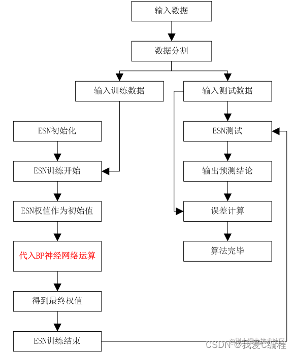
这里,我们的主要方法为:
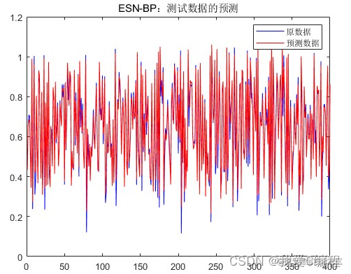
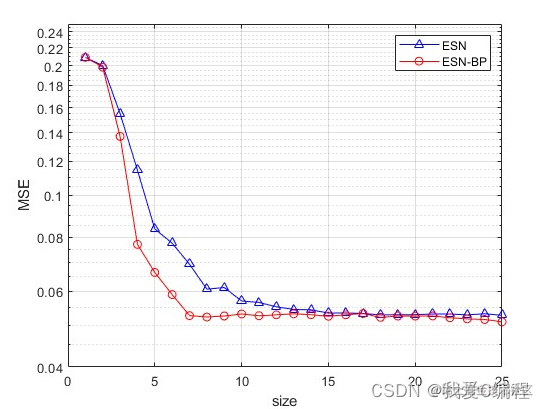
将计算得到的权值作为bp神经网络迭代的初始值,然后以这个初始值为迭代过程的第一个值,不断的训练迭代,最后得到ESN-BP输出的权值,然后进行测试。
下面给出整个算法的流程框图:
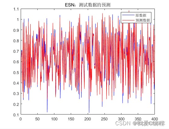
2.仿真效果预览
matlab2022a仿真结果如下:
3.MATLAB核心程序
function esn = generate_esn(nInputUnits, nInternalUnits, nOutputUnits, varargin)

%%%% set the number of units
esn.nInternalUnits = nInternalUnits;
esn.nInputUnits    = nInputUnits;
esn.nOutputUnits   = nOutputUnits;

connectivity = min([10/nInternalUnits 1]);
nTotalUnits = nInternalUnits + nInputUnits + nOutputUnits;

esn.internalWeights_UnitSR = generate_internal_weights(nInternalUnits,connectivity);


esn.nTotalUnits = nTotalUnits;

% input weight matrix has weight vectors per input unit in colums
esn.inputWeights = 2.0 * rand(nInternalUnits, nInputUnits)- 1.0;

% output weight matrix has weights for output units in rows
% includes weights for input-to-output connections
esn.outputWeights = zeros(nOutputUnits, nInternalUnits + nInputUnits);

%output feedback weight matrix has weights in columns
esn.feedbackWeights = (2.0 * rand(nInternalUnits, nOutputUnits)- 1.0);

%init default parameters
esn.inputScaling  = ones(nInputUnits, 1);
esn.inputShift    = zeros(nInputUnits, 1);
esn.teacherScaling= ones(nOutputUnits, 1);
esn.teacherShift  = zeros(nOutputUnits, 1);
esn.noiseLevel = 0.0 ;
esn.reservoirActivationFunction = 'tanh';
esn.outputActivationFunction = 'identity' ; % options: identity or tanh or sigmoid01
esn.methodWeightCompute = 'pseudoinverse' ; % options: pseudoinverse and wiener_hopf
esn.inverseOutputActivationFunction = 'identity' ;
esn.spectralRadius = 1 ;
esn.feedbackScaling = zeros(nOutputUnits, 1);
esn.trained = 0 ;
esn.type = 'plain_esn' ;
esn.timeConstants = ones(esn.nInternalUnits,1);
esn.leakage = 0.5;
esn.learningMode = 'offline_singleTimeSeries' ;
esn.RLS_lambda = 1 ;

args = varargin;
nargs= length(args);
for i=1:2:nargs
  switch args{i},
   case 'inputScaling', esn.inputScaling = args{i+1} ;
   case 'inputShift', esn.inputShift= args{i+1} ;
   case 'teacherScaling', esn.teacherScaling = args{i+1} ;
   case 'teacherShift', esn.teacherShift = args{i+1} ;
   case 'noiseLevel', esn.noiseLevel = args{i+1} ;
   case 'learningMode', esn.learningMode = args{i+1} ;
   case 'reservoirActivationFunction',esn.reservoirActivationFunction=args{i+1};
   case 'outputActivationFunction',esn.outputActivationFunction= args{i+1};
   case 'inverseOutputActivationFunction', esn.inverseOutputActivationFunction=args{i+1};
   case 'methodWeightCompute', esn.methodWeightCompute = args{i+1} ;
   case 'spectralRadius', esn.spectralRadius = args{i+1} ;
   case 'feedbackScaling',  esn.feedbackScaling = args{i+1} ;
   case 'type' , esn.type = args{i+1} ;
   case 'timeConstants' , esn.timeConstants = args{i+1} ;
   case 'leakage' , esn.leakage = args{i+1} ;
   case 'RLS_lambda' , esn.RLS_lambda = args{i+1};
   case 'RLS_delta' , esn.RLS_delta = args{i+1};

   otherwise error('the option does not exist');
  end
end

load data.mat
%数据分割
train_fraction                           = 0.5;
[trainInputSequence, testInputSequence]  = split_train_test(inputSequence,train_fraction);
[trainOutputSequence,testOutputSequence] = split_train_test(outputSequence,train_fraction);

%generate an esn
global nInputUnits;
global nInternalUnits;
global nOutputUnits;
nInputUnits          = 2;
nInternalUnits       = 8;
nOutputUnits         = 1;
esn                  = generate_esn(nInputUnits,nInternalUnits,nOutputUnits,'spectralRadius',0.5,'inputScaling',[0.1;0.1],'inputShift',[0;0],'teacherScaling',[0.3],'teacherShift',[-0.2],'feedbackScaling',0,'type','plain_esn');
esn.internalWeights  = esn.spectralRadius * esn.internalWeights_UnitSR;

%train the ESN
%discard the first 100 points
nForgetPoints        = 100;
%这里,就固定设置一种默认的学习方式,其他的就注释掉了
[trainedEsn,stateMatrix] = train_esn(trainInputSequence,trainOutputSequence,esn,nForgetPoints) ;

%test the ESN
nForgetPoints        = 100 ;
predictedTrainOutput = test_esn(trainInputSequence, trainedEsn, nForgetPoints);
predictedTestOutput  = test_esn(testInputSequence,  trainedEsn, nForgetPoints) ;

figure;
plot(testOutputSequence(nForgetPoints+1:end),'b');
hold on
plot(predictedTestOutput,'r');
legend('原数据','预测数据');
title('ESN-BP:测试数据的预测');


 浙公网安备 33010602011771号