基于LMS自适应滤波的盲信道估计matlab仿真,调制方式为QPSK
1.算法描述
自适应滤波器由参数可调的数字滤波器和自适应算法两部分组成。如图所示。
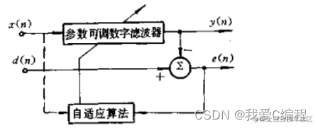
输入信号x(n) 通过参数可调数字滤波器后产生输出信号 y(n),将其与期望信号d(n)进行比较,形成误差信号e(n), 通过自适应算法对滤波器参数进行调整,最终使 e(n)的均方值最小。自适应滤波可以利用前一时刻已得的滤波器参数的结果,自动调节当前时刻的滤波器参数,以适应信号和噪声未知的或随时间变化的统计特性,从而实现最优滤波。自适应滤波器实质上就是一种能调节自身传输特性以达到最优的维纳滤波器。自适应滤波器不需要关于输入信号的先验知识,计算量小,特别适用于实时处理。维纳滤波器参数是固定的,适合于平稳随机信号。卡尔曼滤波器参数是时变的,适合于非平稳随机信号。然而,只有在信号和噪声的统计特性先验已知的情况下,这两种滤波技术才能获得最优滤波。在实际应用中,常常无法得到信号和噪声统计特性的先验知识。在这种情况下,自适应滤波技术能够获得极佳的滤波性能,因而具有很好的应用价值。
信道估计的目的就是估计信道的时域或频域响应,对接收到的数据进行校正和恢复,以获得相干检测的性能增益(可达 3dB)
相干OFDM系统的接收端使用相干检测技术,系统需要知道信道状态信息CSI(Channel State Information)以对接收信号进行信道均衡,从而信道估计成为系统接收端一个重要的环节。在具有多个发射天线的系统中,如果系统发射端使用了空时编码,接收端进行空时译码时,需要知道每一对发射天线与接收天线之间的CSI。而CSI可以通过信道估计获得。
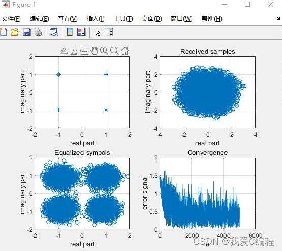
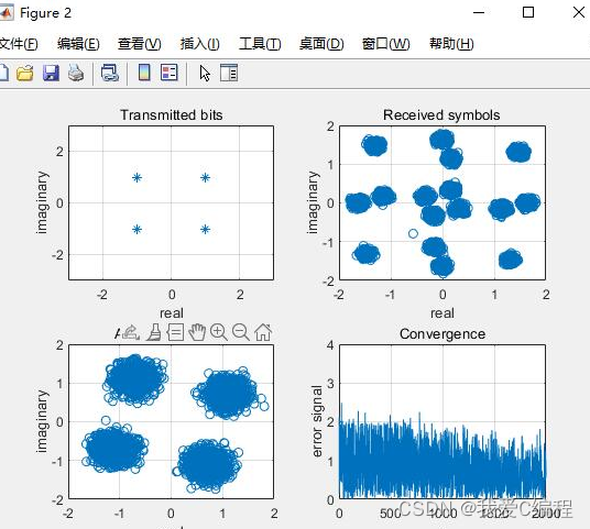
2.仿真效果预览
matlab2022a仿真如下:
3.MATLAB核心程序
x=filter(Ch,1,TxS);  %channel distortion
n=randn(1,M);  %+sqrt(-1)*randn(1,M);   %Additive white gaussian noise
 n=n/norm(n)*10^(-dB/20)*norm(x);  % scale the noise power in accordance with SNR
x=x+n;                           % received noisy signal

K=M-L;   %% Discarding several starting samples for avoiding 0's and negative
X=zeros(L+1,K);  % each vector column is a sample
for i=1:K
    X(:,i)=x(i+L:-1:i).';
end

%adaptive LMS Equalizer
e=zeros(1,T-10);  % initial error
c=zeros(L+1,1);   % initial condition
mu=0.001;        % step size
for i=1:T-10
    e(i)=TxS(i+10+L-EqD)-c'*X(:,i+10);   % instant error
    c=c+mu*conj(e(i))*X(:,i+10);           % update filter or equalizer coefficient
end
sb=c'*X;   % recieved symbol estimation

%SER(decision part)
sb1=sb/norm(c);  % normalize the output
sb1=sign(real(sb1))+sqrt(-1)*sign(imag(sb1));  %symbol detection
start=7;
sb2=sb1-TxS(start+1:start+length(sb1));  % error detection
SER=length(find(sb2~=0))/length(sb2); %  SER calculation
disp(SER);
figure;
% plot of transmitted symbols
    subplot(2,2,1),
    plot(TxS,'*');
    grid,title('Input symbols');  xlabel('real part'),ylabel('imaginary part')
    axis([-2 2 -2 2])

% plot of received symbols
    subplot(2,2,2),
    plot(x,'o');
    grid, title('Received samples');  xlabel('real part'), ylabel('imaginary part')

% plots of the equalized symbols
    subplot(2,2,3),
    plot(sb,'o');
    grid, title('Equalized symbols'), xlabel('real part'), ylabel('imaginary part')

% convergence
    subplot(2,2,4),
    plot(abs(e));
    grid, title('Convergence'), xlabel('n'), ylabel('error signal')
    %%


clc;
clear all;

N=6000;    % number of sample data
dB=25;     % Signal to noise ratio(dB)

L=20; % smoothing length L+1
ChL=1;  % length of the channel= ChL+1
EqD=round((L+ChL)/2);  %  channel equalization delay

i=sqrt(-1);
%Ch=randn(1,ChL+1)+sqrt(-1)*randn(1,ChL+1);   % complex channel

%Ch=[0.0545+j*0.05 .2832-.1197*j -.7676+.2788*j -.0641-.0576*j .0566-.2275*j .4063-.0739*j];
Ch=[0.8+i*0.1 .9-i*0.2]; %complex channel
    Ch=Ch/norm(Ch);% normalize
TxS=round(rand(1,N))*2-1;  % QPSK symbols are transmitted symbols
TxS=TxS+sqrt(-1)*(round(rand(1,N))*2-1);
x=filter(Ch,1,TxS); %channel distortion

n=randn(1,N)+sqrt(-1)*randn(1,N);   % additive white gaussian noise (complex)
 n=n/norm(n)*10^(-dB/20)*norm(x);  % scale noise power
x1=x+n;  % received noisy signal

%estimation using CMA
K=N-L;   %% Discard initial samples for avoiding 0's and negative
X=zeros(L+1,K);  %each vector
for i=1:K
    X(:,i)=x1(i+L:-1:i).';
end

e=zeros(1,K);  % to store the error signal
c=zeros(L+1,1); c(EqD)=1;    % initial condition
R2=2;                  % constant modulous of QPSK symbols
mu=0.001;      % step size
for i=1:K
   e(i)=abs(c'*X(:,i))^2-R2;                  % initial error
   c=c-mu*2*e(i)*X(:,i)*X(:,i)'*c;     % update equalizer co-efficients
   c(EqD)=1;
end

sym=c'*X;   % symbol estimation
%calculate SER
H=zeros(L+1,L+ChL+1); for i=1:L+1, H(i,i:i+ChL)=Ch; end  % channel matrix
fh=c'*H; % channel equalizer
temp=find(abs(fh)==max(abs(fh))); %find maximum
A95

 浙公网安备 33010602011771号