《机器学习十讲》第六讲总结

　　源地址（相关案例在视频下方）：http://cookdata.cn/auditorium/course_room/10017/

《机器学习十讲》——第六讲（降维）

       数学知识

特征向量：设A是n阶方阵，如果有常数λ和n维非零列向量α的关系式Aα=λα成立，则称λ为方阵A的特征值，非零向量α称为方阵A的对应于特征值λ的特征向量。

特征值分解：

在python中使用numpy工具就可以实现。

       降维

定义：将数据的特征数量从高维转换为低维。

作用：解决高维数据的维度灾难问题的一种手段；能够作为一种特征抽取方法；便于对数据进行可视化分析。

       降维方法

主成分分析（PCA）

基本思想：构造原始特征的一系列线性组合形成的线性无关低维特征，以去除数据的相关性，并使降维后的数据最大程度地保持原始高维数据的方差信息。

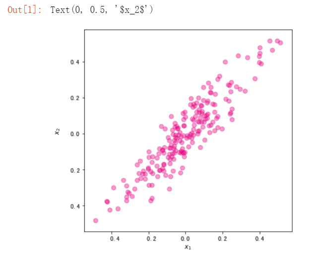
例：二维数据投影到一维（图示）：

数据集表示：

数据集D={x1,x2,…,xn}，每个样本表示成d维向量，且每个维度均为连续型特征。数据集D也可以表示成一个n×d的矩阵X。为方便描述，进一步假设每一维特征的均值均为0（中心化处理），且使用一个d×l的线性转换矩阵W来表示将d维的数据降到l维（l<d）空间的过程，降维后的数据用Y表示，有Y=XW。

优化目标：降维后数据的方差：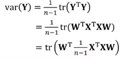

 

 原始数据集的协方差矩阵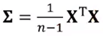，则PCA的数学模型为：

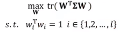
模型求解：

 

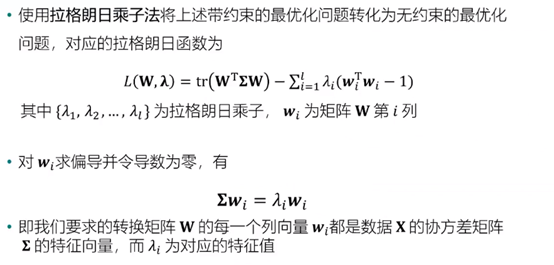
做出以上处理之后，我们还需要将方差最大化：

 

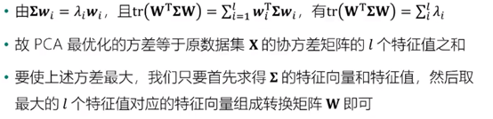
取l个特征值时首先进行降序排序处理。

算法流程：

 

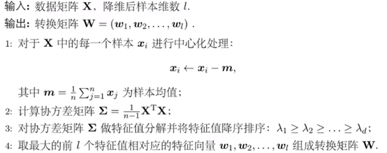
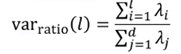
l的选择：

方差比例：通过确定降维前后方差保留比例选择降维后的样本维数l，可预先设置一个方差比例阈值（如90%），公式如下：

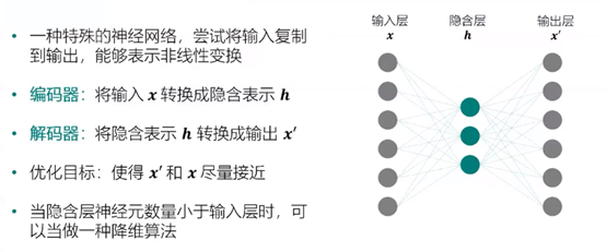
自编码器：

 

 深层自编码器：

　　实例：

Python实现PCA算法：

import numpy as np
#PCA算法
def principal_component_analysis(X, l):
    X = X - np.mean(X, axis=0)#对原始数据进行中心化处理
    sigma = X.T.dot(X)/(len(X)-1) # 计算协方差矩阵
    a,w = np.linalg.eig(sigma) # 计算协方差矩阵的特征值和特征向量
    sorted_indx = np.argsort(-a) # 将特征向量按照特征值进行排序
    X_new = X.dot(w[:,sorted_indx[0:l]])#对数据进行降维****Y=XW
    return X_new,w[:,sorted_indx[0:l]],a[sorted_indx[0:l]] #返回降维后的数据、主成分、对应特征值

from sklearn import datasets
import matplotlib.pyplot as plt
%matplotlib inline
#使用make_regression生成用于线性回归的数据集
x, y = datasets.make_regression(n_samples=200,n_features=1,noise=10,bias=20,random_state=111)
##将自变量和标签进行合并，组成一份二维数据集。同时对两个维度均进行归一化。
x = (x - x.mean())/(x.max()-x.min())
y = (y - y.mean())/(y.max()-y.min())
###可视化展示
fig, ax = plt.subplots(figsize=(6, 6)) #设置图片大小
ax.scatter(x,y,color="#E4007F",s=50,alpha=0.4)
plt.xlabel("$x_1$")
plt.ylabel("$x_2$")

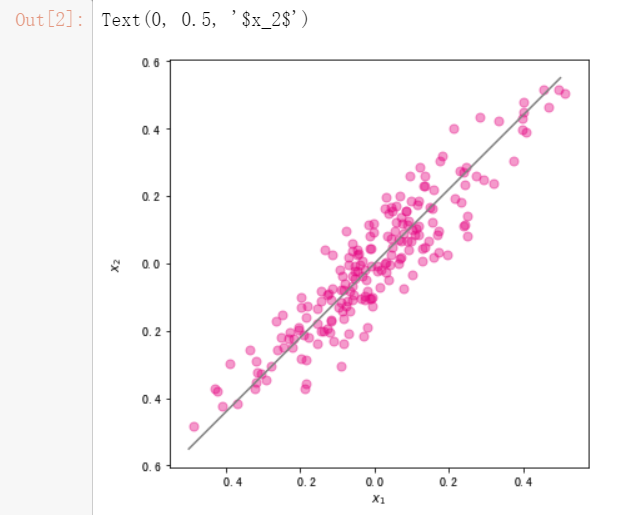
#调用刚才写好的PCA算法对数据进行降维
import pandas as pd
X = pd.DataFrame(x,columns=["x1"])
X["x2"] = y
X_new,w,a = principal_component_analysis(X,1)
#直线的斜率为w[1,0]/w[0,0]。将主成分方向在散点图中绘制出来
import numpy as np
x1 = np.linspace(-.5, .5, 50)
x2 = (w[1,0]/w[0,0])*x1 
fig, ax = plt.subplots(figsize=(6, 6)) #设置图片大小
X = pd.DataFrame(x,columns=["x1"])
X["x2"] = y
ax.scatter(X["x1"],X["x2"],color="#E4007F",s=50,alpha=0.4)
ax.plot(x1,x2,c="gray") # 画出第一主成分直线
plt.xlabel("$x_1$")
plt.ylabel("$x_2$")

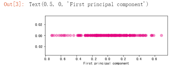
#使用散点图绘制降维后的数据集
import numpy as np
fig, ax = plt.subplots(figsize=(6, 2)) #设置图片大小
ax.scatter(X_new,np.zeros_like(X_new),color="#E4007F",s=50,alpha=0.4)
plt.xlabel("First principal component")

 

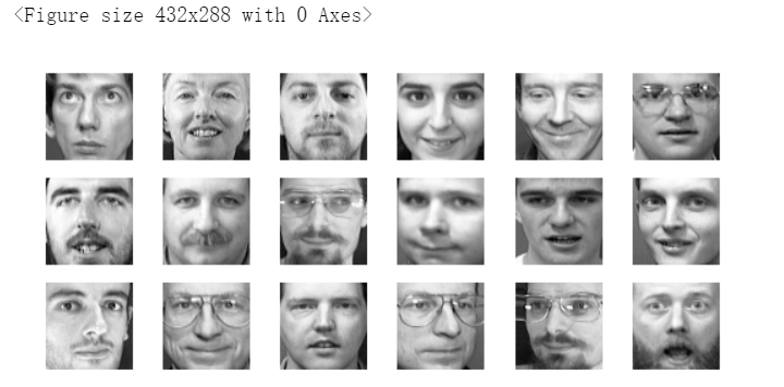
 基于PCA的特征脸提取和人脸重构

#导入olivettifaces人脸数据集
from sklearn.datasets import fetch_olivetti_faces
faces = fetch_olivetti_faces()
faces.data.shape

输出的维度如下

#随机排列
rndperm = np.random.permutation(len(faces.data))
plt.gray()
fig = plt.figure(figsize=(9,4) )
#取18个
for i in range(0,18):
    ax = fig.add_subplot(3,6,i+1 )
    ax.matshow(faces.data[rndperm[i],:].reshape((64,64)))
    plt.box(False) #去掉边框
    plt.axis("off")#不显示坐标轴
plt.show()

#将人脸数据从之前的4096维降低到20维
%time faces_reduced,W,lambdas = principal_component_analysis(faces.data,20)

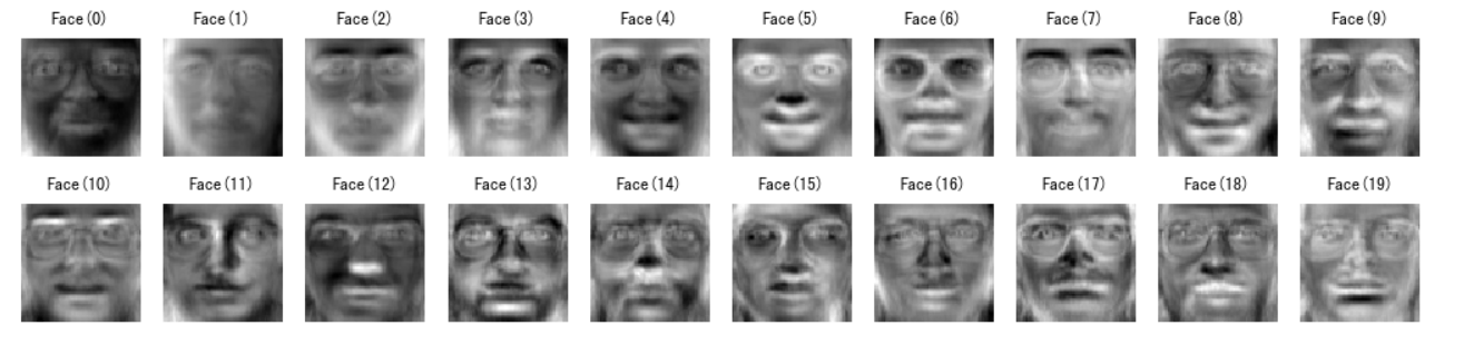
#将降维后得到的20个特征向量表示出来
fig = plt.figure( figsize=(18,4))
plt.gray()
for i in range(0,20):
    ax = fig.add_subplot(2,10,i+1 )
    #将降维后的W每一列都提出，从4096长度向量变成64×64的图像
    ax.matshow(W[:,i].reshape((64,64)))
    plt.title("Face(" + str(i) + ")")
    plt.box(False) #去掉边框
    plt.axis("off")#不显示坐标轴
plt.show()

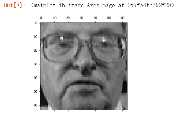
sample_indx = np.random.randint(0,len(faces.data)) #随机选择一个人脸的索引
#显示原始人脸
plt.matshow(faces.data[sample_indx].reshape((64,64)))

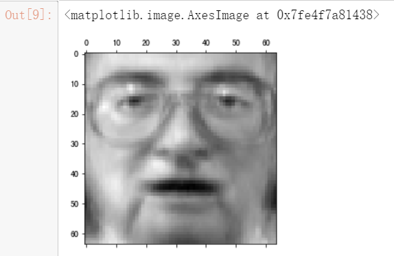
# 显示重构人脸
##matshow(平均脸+降维后的每个维度与W列加权求和)
plt.matshow(faces.data.mean(axis=0).reshape((64,64)) + W.dot(faces_reduced[sample_indx]).reshape((64,64)))

#将重构过程进行可视化展示
fig = plt.figure( figsize=(20,4))
plt.gray()
ax = fig.add_subplot(2,11,1)
ax.matshow(faces.data.mean(axis=0).reshape((64,64))) #显示平均脸
for i in range(0,20):
    ax = fig.add_subplot(2,11,i+2 )
    ax.matshow(W[:,i].reshape((64,64)))
    plt.title( str(round(faces_reduced[sample_indx][i],2)) + "*Face(" + str(i) + ")")
    plt.box(False) #去掉边框
    plt.axis("off")#不显示坐标轴
plt.show()

 

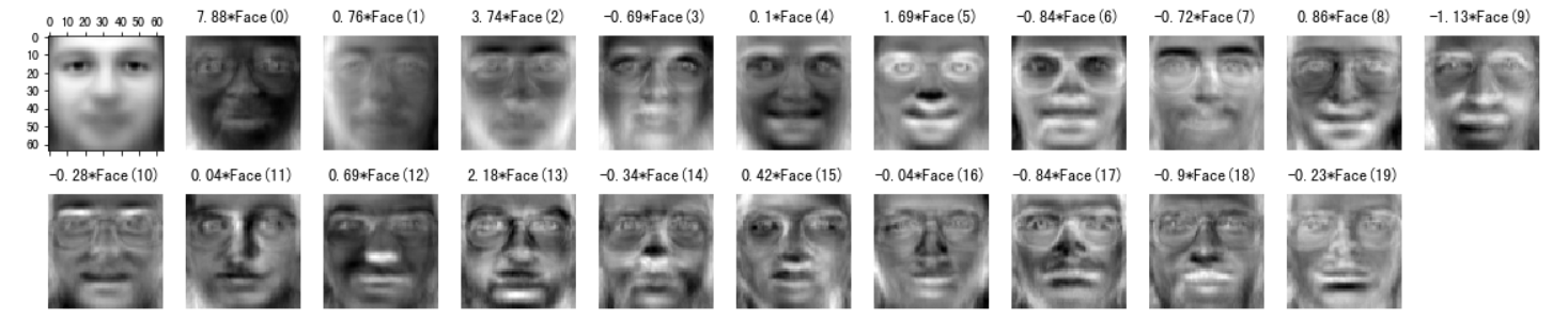
 使用MNIST手写数据集对PCA进行含义理解

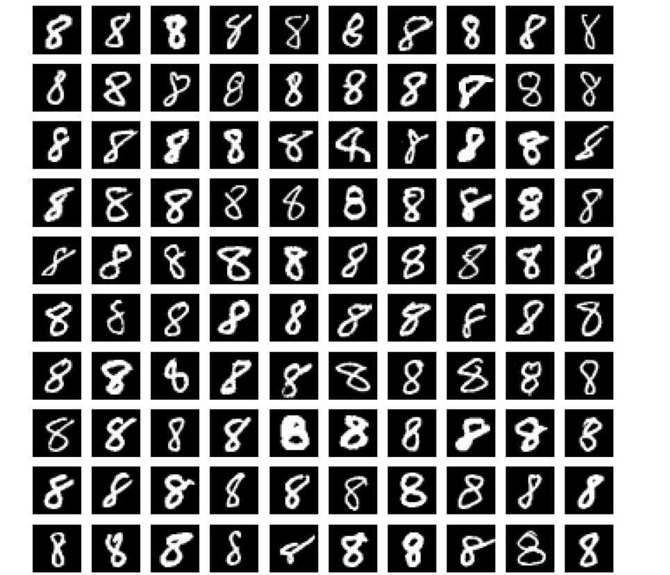
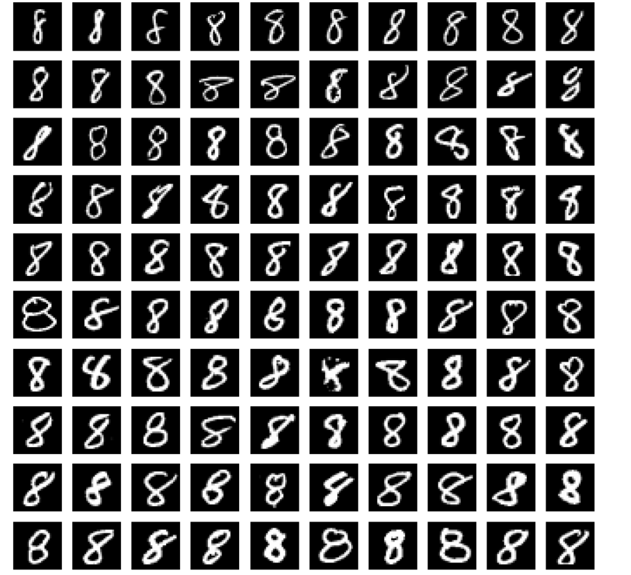
#导入MNIST数据集
import numpy as np
f = np.load("input/mnist.npz") 
X_train, y_train, X_test, y_test = f['x_train'], f['y_train'],f['x_test'], f['y_test']
f.close()
#将图像拉平成784维的向量表示，并对像素值进行归一化。
##原为（60000，28，28），拉平成（60000，784）
x_train = X_train.reshape((-1, 28*28)) / 255.0
x_test = X_test.reshape((-1, 28*28)) / 255.0
#以数字8为例
digit_number = x_train[y_train == 8]
#随机选择一些数据进行可视化
rndperm = np.random.permutation(len(digit_number))
%matplotlib inline
import matplotlib.pyplot as plt
plt.gray()
fig = plt.figure( figsize=(12,12) )
for i in range(0,100):
    ax = fig.add_subplot(10,10,i+1)
    ax.matshow(digit_number[rndperm[i]].reshape((28,28)))
    plt.box(False) #去掉边框
    plt.axis("off")#不显示坐标轴  
plt.show()

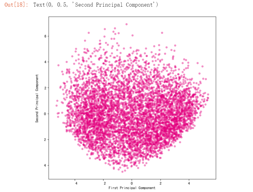
#使用PCA算法将数字8的图片降维至二维
number_reduced,number_w,number_a = principal_component_analysis(digit_number,2)
#可视化
import warnings
warnings.filterwarnings('ignore') #该行代码的作用是隐藏警告信息
import matplotlib.pyplot as plt
%matplotlib inline
fig, ax = plt.subplots(figsize=(8, 8)) #设置图片大小
ax.scatter(number_reduced[:,0],number_reduced[:,1],color="#E4007F",s=20,alpha=0.4)
plt.xlabel("First Principal Component")
plt.ylabel("Second Principal Component")

#将图片从小到大做排序
##观察第一主成分（[:,0]）的结果
sorted_indx = np.argsort(number_reduced[:,0])
plt.gray()
fig = plt.figure( figsize=(12,12) )
for i in range(0,100):
    ax = fig.add_subplot(10,10,i+1)
    #每隔50取一个样本
    ax.matshow(digit_number[sorted_indx[i*50]].reshape((28,28)))
    plt.box(False) #去掉边框
    plt.axis("off")#不显示坐标轴  
plt.show()

 

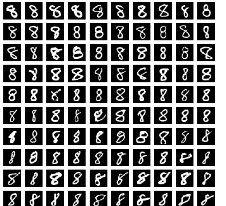
 可以看到数字 8 顺时针倾斜的角度不断加大。第一个主成分的含义很可能代表的就是数字的倾斜角度。

##观察第二主成分（[:,1]）的结果
sorted_indx = np.argsort(number_reduced[:,1])
plt.gray()
fig = plt.figure( figsize=(12,12) )
for i in range(0,100):
    ax = fig.add_subplot(10,10,i+1)
    ax.matshow(digit_number[sorted_indx[i*50]].reshape((28,28)))
    plt.box(False) #去掉边框
    plt.axis("off")#不显示坐标轴  
plt.show()

 

 第二主成分没有第一主成分那么明显，个人猜测与8的手写比例相关。

基于AutoEncoder的图像压缩与重构

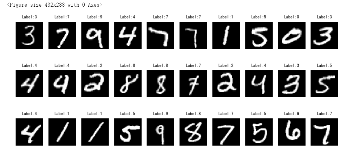
#从MNIST数据集里采样一个图像子集，可视化
rndperm = np.random.permutation(len(X_train))
%matplotlib inline
import matplotlib.pyplot as plt
plt.gray()
fig = plt.figure(figsize=(16,7))
for i in range(0,30):
    ax = fig.add_subplot(3,10,i+1, title='Label:' + str(y_train[rndperm[i]]) )
    ax.matshow(X_train[rndperm[i]])
    plt.box(False) #去掉边框
    plt.axis("off")#不显示坐标轴  
plt.show()

 

 使用Tensorflow构建自编码器

#导入Tensorflow模块
import tensorflow as tf
import tensorflow.keras.layers as layers
#该平台中没有GPU资源，因此使用CPU
print(tf.test.is_gpu_available())

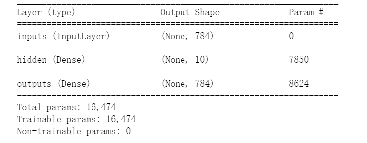
#归一化
x_train = X_train.reshape((-1, 28*28)) / 255.0
x_test = X_test.reshape((-1, 28*28)) / 255.0
#构建自编码器，并打印模型
inputs = layers.Input(shape=(28*28,), name='inputs')
hidden = layers.Dense(10, activation='relu', name='hidden')(inputs)
outputs = layers.Dense(28*28, name='outputs')(hidden)
auto_encoder = tf.keras.Model(inputs,outputs)
auto_encoder.summary()

#使用compile编译
##定义优化算法adam，误差函数mean_squared_error
auto_encoder.compile(optimizer='adam',loss='mean_squared_error')
#使用fit训练模型
##verbose=1显示训练过程，verbose=0维隐藏训练过程
%time auto_encoder.fit(x_train, x_train, batch_size=100, epochs=100,verbose=0)

因为数据集在此平台内是保存好的，省去了下载的麻烦，所以实战编译直接在此平台内进行，然而出现了训练模型迟迟不出结果的问题。。。。因此仅出示代码

#预测
x_train_pred = auto_encoder.predict(x_train)
# Plot the graph
plt.gray()
fig = plt.figure( figsize=(16,4) )
n_plot = 10
for i in range(n_plot):
    ax1 = fig.add_subplot(2,10,i+1, title='Label:' + str(y_train[rndperm[i]]) )
    ax1.matshow(X_train[rndperm[i]])
    ax2 = fig.add_subplot(2,10,i + n_plot + 1)
    ax2.matshow(x_train_pred[rndperm[i]].reshape((28,28)))
    ax1.get_xaxis().set_visible(False)
    ax1.get_yaxis().set_visible(False)
    ax2.get_xaxis().set_visible(False)
    ax2.get_yaxis().set_visible(False)
plt.show()

由于之前的训练模型没有出结果，预测部分也无法查看效果，下面附上样例中的预测效果图，如果执行顺利差别应该不大。。。

 

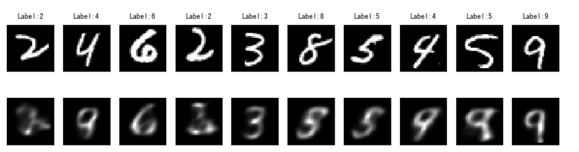
 可见样例中自编码器最后得到的模型并不是太好，因此接下来构建多层自编码器。该部分其实在早期的日报博客中已经有所涉猎（多个Dense层）：

#添加多个Dense层
inputs = layers.Input(shape=(28*28,), name='inputs')
hidden1 = layers.Dense(200, activation='relu', name='hidden1')(inputs)
hidden2 = layers.Dense(50, activation='relu', name='hidden2')(hidden1)
hidden3 = layers.Dense(10, activation='relu', name='hidden3')(hidden2)
hidden4 = layers.Dense(50, activation='relu', name='hidden4')(hidden3)
hidden5 = layers.Dense(200, activation='relu', name='hidden5')(hidden4)
outputs = layers.Dense(28*28, activation='softmax', name='outputs')(hidden5)
deep_auto_encoder = tf.keras.Model(inputs,outputs)
deep_auto_encoder.summary()

deep_auto_encoder.compile(optimizer='adam',loss='binary_crossentropy') #定义误差和优化方法
%time deep_auto_encoder.fit(x_train, x_train, batch_size=100, epochs=200,verbose=1) #模型训练

训练过程依然出现了问题，怀疑是网络连接，因为之前报了无法连接本地服务器之后才开始没动静的：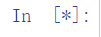

x_train_pred2 = deep_auto_encoder.predict(x_train)
# Plot the graph
plt.gray()
fig = plt.figure( figsize=(16,3) )
n_plot = 10
for i in range(n_plot):
    ax1 = fig.add_subplot(2,10,i+1, title='Label:' + str(y_train[rndperm[i]]) )
    ax1.matshow(X_train[rndperm[i]])
    ax3 = fig.add_subplot(2,10,i + n_plot + 1 )
    ax3.matshow(x_train_pred2[rndperm[i]].reshape((28,28)))
    ax1.get_xaxis().set_visible(False)
    ax1.get_yaxis().set_visible(False)
    ax3.get_xaxis().set_visible(False)
    ax3.get_yaxis().set_visible(False)
plt.show()

这里还是展示样例图：

 

 实战——中文新闻数据降维与可视化

#引入数据，因为是中文所以要设置encoding参数为utf8，sep参数为\t
import pandas as pd
news = pd.read_csv("./input/chinese_news_cutted_train_utf8.csv",sep="\t",encoding="utf8")
#加载停用词
stop_words = []
file = open("./input/stopwords.txt") 
for line in file:
    stop_words.append(line.strip())
file.close()

from sklearn.feature_extraction.text import TfidfVectorizer
vectorizer = TfidfVectorizer(stop_words=stop_words,min_df=0.01,max_df=0.5,max_features=500)
news_vectors = vectorizer.fit_transform(news["分词文章"])
news_df = pd.DataFrame(news_vectors.todense())
#使用PCA将数据降维至二维
from sklearn.decomposition import PCA
pca = PCA(n_components=2)
news_pca = pca.fit_transform(news_df)
#可视化
import seaborn as sns
import matplotlib.pyplot as plt
plt.figure(figsize=(10,10))
sns.scatterplot(news_pca[:,0], news_pca[:,1],hue = news["分类"].values,alpha=0.5)

使用sklearn里的PCA算法，不必再自己写个函数

 

 降维效果不是特别理想。不同主题的新闻在二维空间上互相重叠。因此更新一下降维方法：

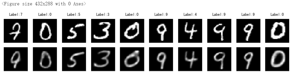
#t-SNE降维方法
from sklearn.manifold import TSNE
#先降到20维
pca10 = PCA(n_components=20)
news_pca10 = pca10.fit_transform(news_df)
#再降到2维
tsne_news = TSNE(n_components=2, verbose=1)
#输出运行时间
%time tsne_news_results = tsne_news.fit_transform(news_pca10)
#可视化
plt.figure(figsize=(10,10))
sns.scatterplot(tsne_news_results[:,0], tsne_news_results[:,1],hue = news["分类"].values,alpha=0.5)

 

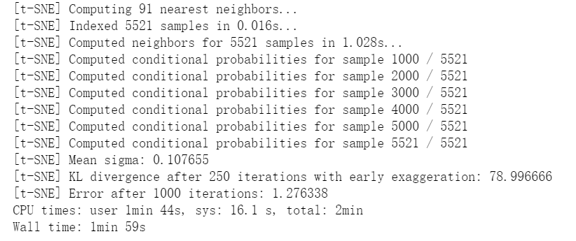
 t-SNE运行时间较慢，因此要先进行一步降维操作，将维度降低至20维，再换t-SNE方法，节省时间

最后可视化效果如下：

 

 可见效果更好一些。