《机器学习十讲》第二讲总结

　　源地址（相关案例在视频下方）：http://cookdata.cn/auditorium/course_room/10013/

　　第二讲的主要内容是回归，总结如下。

　　回归模型用了很多的矩阵知识，因此首先回顾一下矩阵知识以及python中的使用：

矩阵的逆：

若A为可逆矩阵，则逆矩阵是唯一的。

判断矩阵是否可逆：行列式不等于0；满秩；行或列向量组线性无关。

#求逆矩阵
import numpy as np
#格式化numpy输出
np.set_printoptions(formatter={'float':'{: 0.2f}'.format})
A = np.array([[4,5,1],[0,8,3],[9,4,7]])
#求行列式
print("行列式："+str(np.linalg.det(A)))
#求逆
B = np.linalg.inv(A)
print("A的逆矩阵B")
print(B)
#结果验证
print("BA：")
print(B.dot(A))
print("AB：")
print(A.dot(B))

 

 

 .dot，.inv都是后面经常用到的东西，下面进入回归正题。

回归：

概述：最早由英国生物统计学家高尔顿和他的学生皮尔逊在研究父母亲和子女的身高遗传特性时提出，如今指用一个或多个自变量来预测因变量的·数学方法。在机器学习中，回归指的是一类预测变量为连续值的有监督学习方法。

因变量：需要预测的变量（Y）

自变量：解释因变量变化的变量（X）

 

一元线性回归：

模型：y=w1*x+w0，其中w0，w1为回归系数

说明：给定训练集D={(x1,y1),…,(xn,yn)}，我们的目标是找到一条直线y=w1*x+w0使得所有样本尽可能落在它的附近。

优化目标（均方误差）：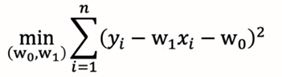

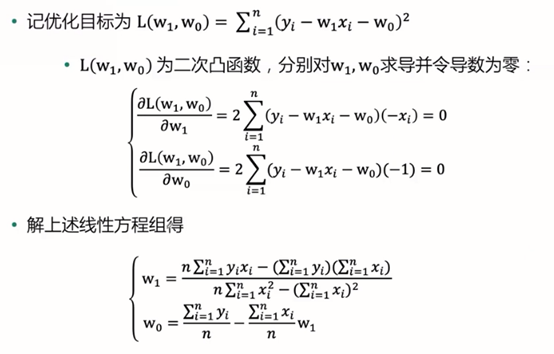
求解：

 

 

 

多元线性回归：

模型：y是多个特征的线性组合：y=w1*x1+w2*x2+…+wd*xd+w0

训练集：D={(x1,y1),…,(xn,yn)},

补充：xi为d维特征向量xi=(x11,x12,…,x1d)^T，设模型对xi的预测值为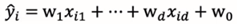

优化目标（最小化均方误差）：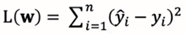

注：寻找一个超平面，使得训练集中样本到超平面的误差平方和最小。

矩阵表示：

假设训练集特征部分记为n*(d+1)矩阵X，最后一列取值全为1。

标签部分记为y=(y1,y2,…,yn)^T，参数记为w=(w1,w2,…,wd,w0)^T。

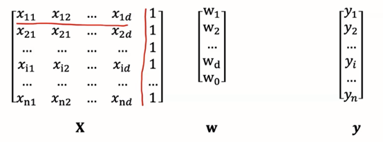
多元线性回归模型就可以表示成下列形式：

优化目标的矩阵表示如下：

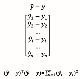
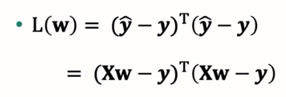
其中w是未知量，X和y是已知量（训练集）。

将优化目标矩阵表示之后，可以进行参数估计：

 

 

线性回归问题：

问题1：实际数据可能不是线性的。

解决方法：多项式回归：使用原始特征的二次项，三次项。问题在于会发生维度灾难，过度拟合。

问题2：多重共线性。

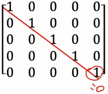
奇异：将X^TX展开时，由于共线性问题，极端情况下会有两行（列）是一样的。

解决方法：最简单的解决方法是在发生共线性的数据中仅选择一个，或者使用正则化，主成分回归，偏最小二乘回归。

问题3：过度拟合问题：当模型变量过多时，线性回归可能会出现过度拟合问题。

解决方法：正则化：

后加的项称为正则项或惩罚函数，λ是自定义的超参数。q=2时：岭回归；q=1时：LASSO。

 

正则化模型介绍：

岭回归：目标函数：

 

 

对w求导并令导数等于0易得：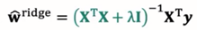

 

 

注意在线性回归目标函数中w包括了w1-w0，而惩罚项中w里不包括w0，只包括w1-wd。

因此在求得结果中单位矩阵I的右下角处1改为0：

 

岭迹：当不断增大正则化参数λ，估计参数（岭回归系数）

在坐标系上的变化曲线称为岭迹。岭迹波动很大，说明该变量有共线性。可根据岭迹做超参数λ的选择。

————————————————————————————————————————————————

LASSO：一种系数压缩估计方法，基本思想是通过追求稀疏性自动选择重要的变量。

目标函数：

注：LASSO的解没有表达式，常用的求解算法包括坐标下降法，LARS算法，ISTA算法等。

 

岭回归与LASSO：

图示1

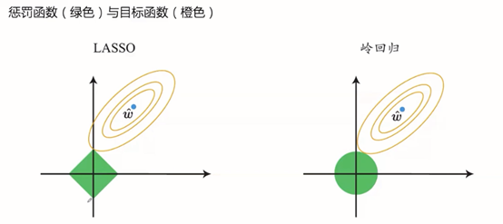
相切值为最优点，LASSO的特点在于取最优点时，横坐标（设为w1）w1=0，而岭回归不是。

图示2——正则化路径

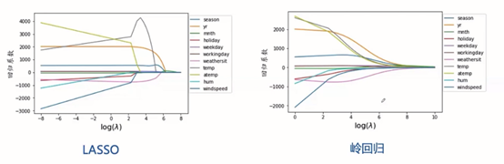
随着λ增大，LASSO的特征系数逐个减小为0，可以做特征选择；岭回归变量系数几乎同时趋近于0。

 

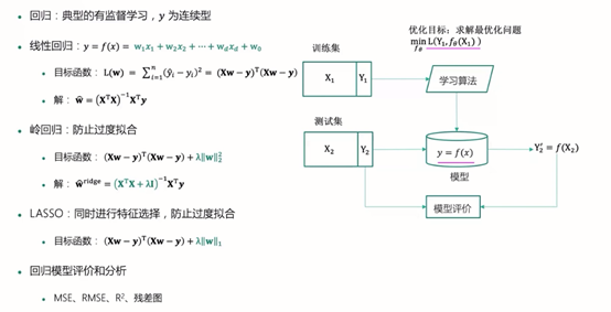
回归模型的评价指标：

 

 

 

 

 

 

案例——使用回归模型预测鲍鱼年龄。

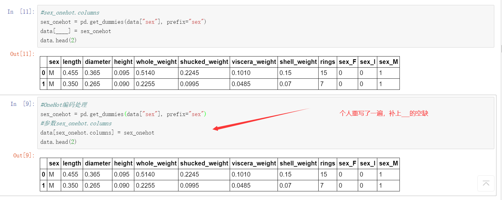
因为案例直接保存在“我的案例”中，里面已经有了相关代码，但有些地方设置成了“___”，需要自行填充，因此我会附上填充后的源码与运行截图，大部分代码和示例代码是相同的：

先发个图说明一下情况，下面是的代码是我新开了一个代码块再写了一遍：

 

 

 接下来进入正题

#首先将数据集引入
import pandas as pd
import warnings
warnings.filterwarnings('ignore')
data = pd.read_csv("./input/abalone_dataset.csv")
#输出前五行
data.head()

#查看数据集中样本数量和特征数量
data.shape

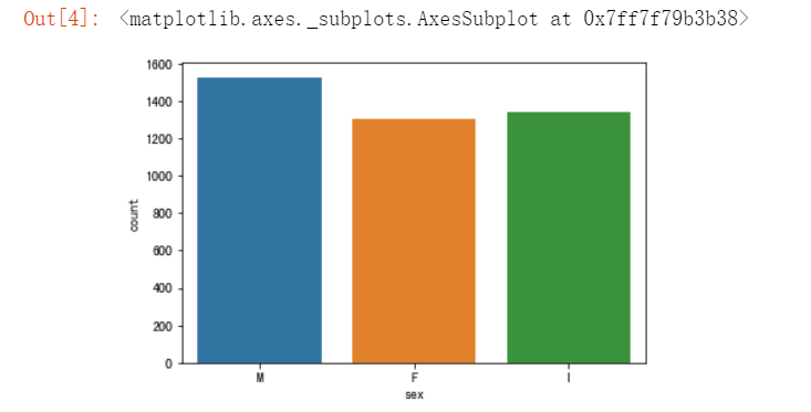
#使用seaborn绘制sex的取值分布条形图
import seaborn as sns
import matplotlib.pyplot as plt
%matplotlib inline
sns.countplot(x = "sex", data = data)

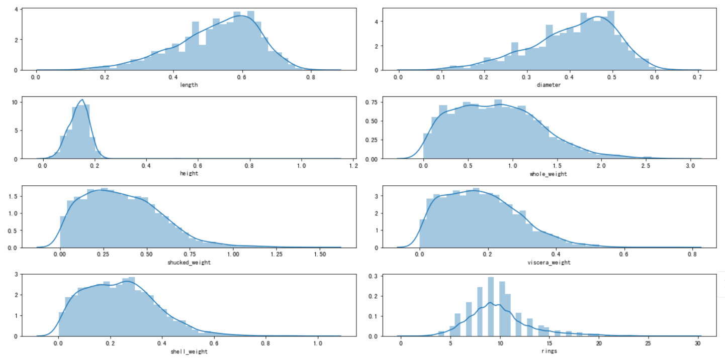
#绘制直方图观察特征取值
i = 1 # 子图记数
plt.figure(figsize=(16, 8))
for col in data.columns[1:]:
    plt.subplot(4,2,i)
    i = i + 1
    sns.distplot(data[col])  
plt.tight_layout()

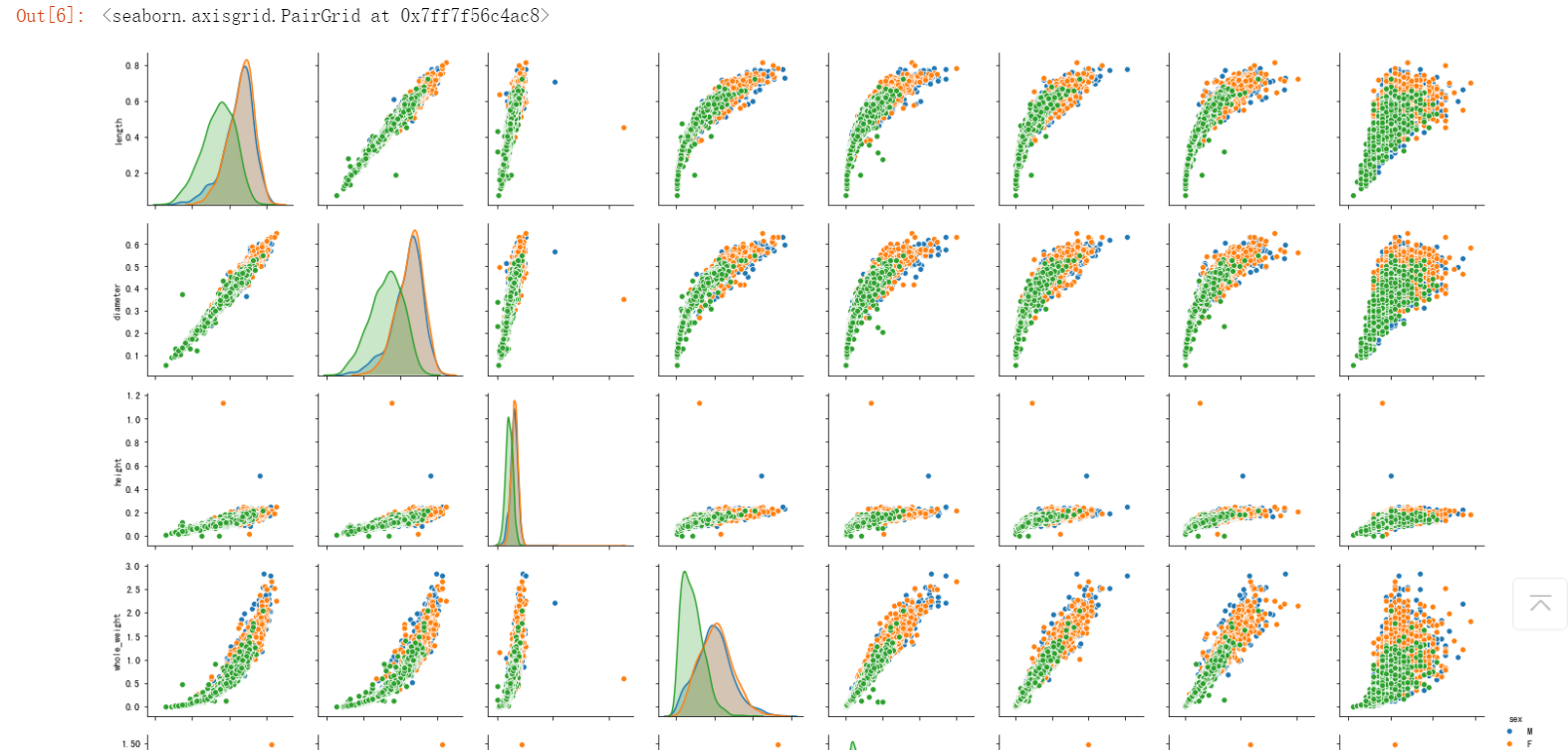
#根据sex画出不同特征之间的点缀图，seaborn提供了pairplot方法
sns.pairplot(data,hue="sex")

 

 

 

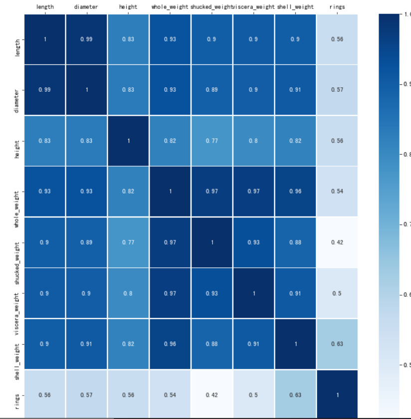
#计算特征之间的相关性
corr_df = data.corr()
corr_df

#为了能够直观看出关系，可以绘制热力图
fig, ax = plt.subplots(figsize=(12, 12))
#原图是绿色的，这里改成蓝色
ax = sns.heatmap(corr_df,linewidths=.5,cmap="Blues",annot=True,xticklabels=corr_df.columns, yticklabels=corr_df.index)
ax.xaxis.set_label_position('top') 
ax.xaxis.tick_top()

#OneHot编码处理
sex_onehot = pd.get_dummies(data["sex"], prefix="sex")
#参数sex_onehot.columns
data[sex_onehot.columns] = sex_onehot
data.head(2)

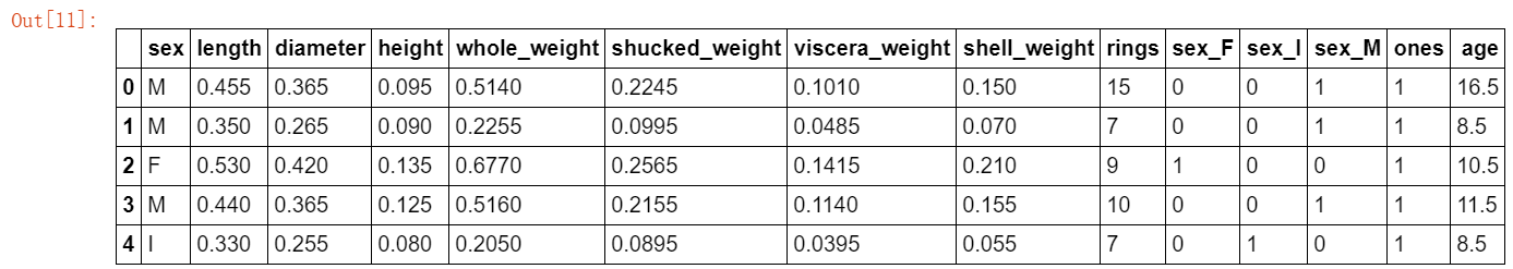
#添加取值为1的特征列
data["ones"] = 1
data.head(5)

 

 

 一般每过一年，鲍鱼就会在其壳上留下一道深深的印记，这叫生长纹，就相当于树木的年轮。在本数据集中，我们要预测的是鲍鱼的年龄，可以通过环数 rings 加上 1.5 得到。所以：

#令age=rings+1.5
data["age"] = data["rings"] + 1.5
data.head(5)

 

 

 将预测目标设置为 age 列，然后构造两组特征，一组包含 ones，一组不包含 ones 。对于 sex 相关的列，我们只使用 sex_F 和 sex_M。后面的模型比对中是否使用数据集的ones列会出现分歧，因此要提前分好。

#构造特征集
y = data["age"]
features_with_ones = ["length","diameter","height","whole_weight","shucked_weight","viscera_weight","shell_weight","sex_F","sex_M","ones"]
features_without_ones=["length","diameter","height","whole_weight","shucked_weight","viscera_weight","shell_weight","sex_F","sex_M"]
X = data[features_with_ones]

#训练集与测试集切分train_test_split
from sklearn import model_selection
X_train,X_test,y_train,y_test = model_selection.train_test_split(X,y,test_size=0.2, random_state=111)

首先是线性回归：

公式及参数说明如下：

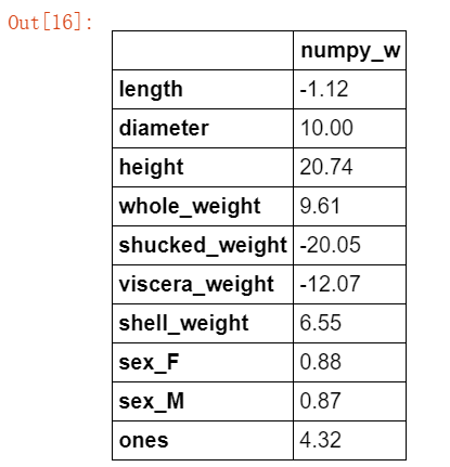
#根据公式补充参数
import numpy as np
def linear_regression(X,y):
    w = np.zeros_like(X.shape[1])
    if np.linalg.det(X.T.dot(X)) != 0 :
        w = np.linalg.inv(X.T.dot(X)).dot(X.T).dot(y)
    return w

#根据模型获取系数
w1 = linear_regression(X_train,y_train)
w1 = pd.DataFrame(data = w1,index = X.columns,columns = ["numpy_w"])
w1.round(decimals=2)

 

 

 这里偷个懒，直接附上案例中的说明，sklearn后面要用到多次：

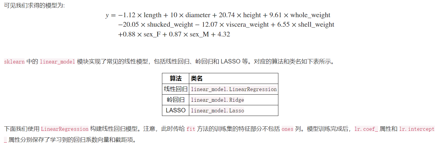
#使用之前介绍的sklearn作系数比对
from sklearn import linear_model
lr = linear_model.LinearRegression()
#刚才处理的时候将新设置的ones放了进去，而这里使用时不能添加ones列
lr.fit(X_train[features_without_ones],y_train)
w_lr = []
w_lr.extend(lr.coef_)
w_lr.append(lr.intercept_)
w1["lr_sklearn_w"] = w_lr
w1.round(decimals=2)

 

 

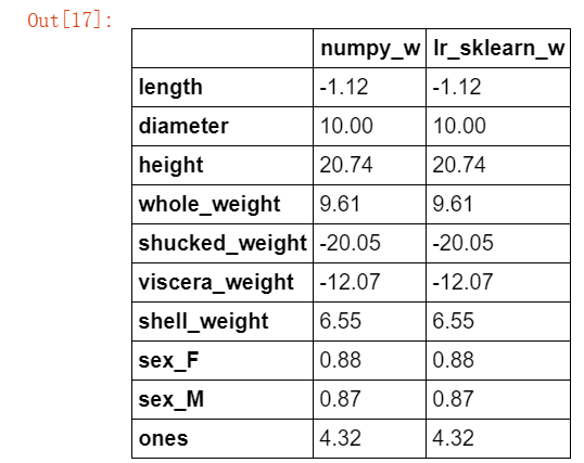
 对比效果是一致的，证明模型构建成功。

 

岭回归：

公式及参数说明：

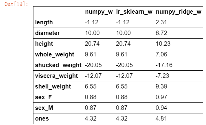
def ridge_regression(X,y,ridge_lambda):
    #eye方法：生成单位矩阵
    penality_matrix = np.eye(X.shape[1])
    #令单位矩阵的最后一个元素=0
    penality_matrix[X.shape[1] - 1][X.shape[1] - 1] = 0
    #输入参数
    w = np.linalg.inv(X.T.dot(X) + ridge_lambda*penality_matrix).dot(X.T).dot(y)
    return w

#使用岭回归模型，与之前两个模型进行比对
w2 = ridge_regression(X_train,y_train,1.0)
w1["numpy_ridge_w"] = w2
w1.round(decimals=2)

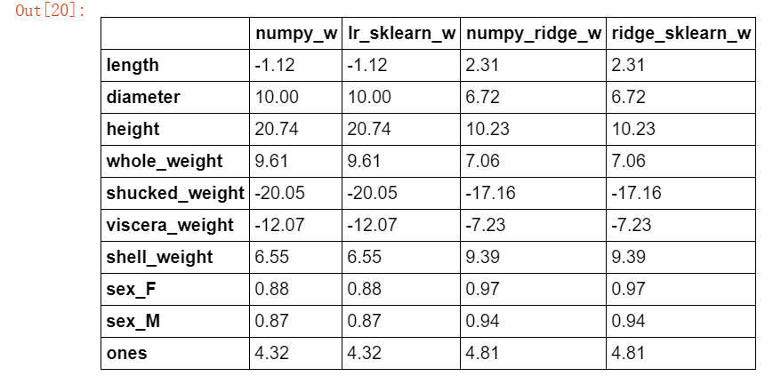
#再与sklearn中的岭回归进行对比
from sklearn.linear_model import Ridge
ridge = linear_model.Ridge(alpha=1.0)
#这里还是使用无ones列的数据集
ridge.fit(X_train[features_without_ones],y_train)
w_ridge = []
w_ridge.extend(ridge.coef_)
w_ridge.append(ridge.intercept_)
w1["ridge_sklearn_w"] = w_ridge
w1.round(decimals=2)

 

 

 

LASSO：

LASSO的解没有公式（上面已经提到过），因此直接使用函数构建：

#使用LASSO
from sklearn.linear_model import Lasso
#alpha设置要小一些，否则
lasso = linear_model.Lasso(alpha=1)
lasso.fit(X_train[features_without_ones],y_train)
print(lasso.coef_)
print(lasso.intercept_)

 

 

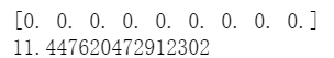
上边示范一下当alpha参数设置过大时的情况

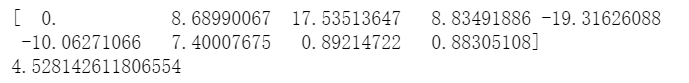
因此设置适当的值：

from sklearn.linear_model import Lasso
#因此设置0.001，设置值越小压缩越小，因为这次案例使用的数据集容量本就不多
lasso = linear_model.Lasso(alpha=0.001)
lasso.fit(X_train[features_without_ones],y_train)
print(lasso.coef_)
print(lasso.intercept_)

 

 

 

模型评估：

MAE：

#平均绝对误差MAE
##使用sklearn.metrics进行预测
from sklearn.metrics import mean_absolute_error
#线性回归
y_test_pred_lr = lr.predict(X_test.iloc[:,:-1])
print(round(mean_absolute_error(y_test,y_test_pred_lr),4))

#岭回归
y_test_pred_ridge = ridge.predict(X_test[features_without_ones])
print(round(mean_absolute_error(y_test,y_test_pred_ridge),4))

#LASSO
y_test_pred_lasso = lasso.predict(X_test[features_without_ones])
print(round(mean_absolute_error(y_test,y_test_pred_lasso),4))

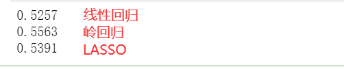
R2：

#决定系数R2
from sklearn.metrics import r2_score
#线性回归
print(round(r2_score(y_test,y_test_pred_lr),4))
#岭回归
print(round(r2_score(y_test,y_test_pred_ridge),4))
#LASSO
print(round(r2_score(y_test,y_test_pred_lasso),4))

 

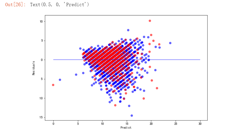
 残差图：

#构建残差图进行诊断
##横轴是模型的预测值，纵轴是预测值与真实值的差距
plt.figure(figsize=(9, 6))
y_train_pred_ridge = ridge.predict(X_train[features_without_ones])
plt.scatter(y_train_pred_ridge, y_train_pred_ridge - y_train, c="b", alpha=0.6)
plt.scatter(y_test_pred_ridge, y_test_pred_ridge - y_test, c="r",alpha=0.6)
plt.hlines(y=0, xmin=0, xmax=30,color="b",alpha=0.6)
plt.ylabel("Residuals")
plt.xlabel("Predict")

 

 岭迹：

#构建岭迹
alphas = np.logspace(-10,10,20)
coef = pd.DataFrame()
for alpha in alphas:
    ridge_clf = Ridge(alpha=alpha)
    ridge_clf.fit(X_train[features_without_ones],y_train)
    df = pd.DataFrame([ridge_clf.coef_],columns=X_train[features_without_ones].columns)
    df['alpha'] = alpha
    coef = coef.append(df,ignore_index=True)
coef.head().round(decimals=2)

 

 

#根据刚才构建好的数据，进行绘图
plt.rcParams['figure.dpi'] = 300 #分辨率
plt.figure(figsize=(9, 6))
coef['alpha'] = coef['alpha']

for feature in X_train.columns[:-1]:
    plt.plot('alpha',feature,data=coef)
ax = plt.gca()
ax.set_xscale('log')
plt.legend(loc='upper right')
plt.xlabel(r'$\alpha$',fontsize=15)
plt.ylabel('系数',fontsize=15)

plt.show()

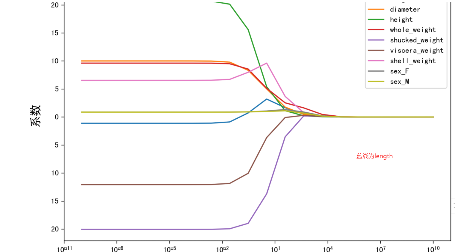
LASSO的正则化路径：

#绘制LASSO的正则化路径
##数据准备
coef = pd.DataFrame()
for alpha in np.linspace(0.0001,0.2,20):
    lasso_clf = Lasso(alpha=alpha)
    lasso_clf.fit(X_train[features_without_ones],y_train)
    df = pd.DataFrame([lasso_clf.coef_],columns=X_train[features_without_ones].columns)
    df['alpha'] = alpha
    coef = coef.append(df,ignore_index=True)
coef.head()
##绘图
plt.figure(figsize=(9, 6))
for feature in X_train.columns[:-1]:
    plt.plot('alpha',feature,data=coef)
plt.legend(loc='upper right')
plt.xlabel(r'$\alpha$',fontsize=15)
plt.ylabel('系数',fontsize=15)
plt.show()

 

 

　　总结：