期末大作业

一、boston房价预测

1. 读取数据集

#1. 读取数据集
from sklearn.datasets import load_boston
data = load_boston()

2. 训练集与测试集划分

#2. 训练集与测试集划分
from sklearn.model_selection import train_test_split
x_train, x_test, y_train, y_test= train_test_split(data.data,data.target,test_size=0.3)

3. 线性回归模型：建立13个变量与房价之间的预测模型，并检测模型好坏。

#3. 线性回归模型：建立13个变量与房价之间的预测模型，并检测模型好坏。
from sklearn.linear_model import LinearRegression
mlr = LinearRegression()
mlr.fit(x_train,y_train)
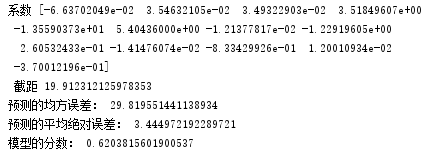
print('系数',mlr.coef_,"\n","截距",mlr.intercept_)
from sklearn.metrics import regression
y_pred = mlr.predict(x_test)
print("预测的均方误差：", regression.mean_squared_error(y_test,y_pred))
print("预测的平均绝对误差：", regression.mean_absolute_error(y_test,y_pred))
print("模型的分数：",mlr.score(x_test, y_test))

　　

4. 多项式回归模型：建立13个变量与房价之间的预测模型，并检测模型好坏。

#4. 多项式回归模型：建立13个变量与房价之间的预测模型，并检测模型好坏。
from sklearn.preprocessing import PolynomialFeatures
a = PolynomialFeatures(degree=2)
x_poly_train = a.fit_transform(x_train)
x_poly_test = a.transform(x_test)
mlrp = LinearRegression()
mlrp.fit(x_poly_train, y_train)
y_pred2 = mlrp.predict(x_poly_test)
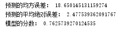
print("预测的均方误差：", regression.mean_squared_error(y_test,y_pred2))
print("预测的平均绝对误差：", regression.mean_absolute_error(y_test,y_pred2))
print("模型的分数：",mlrp.score(x_poly_test, y_test))

　　

5. 比较线性模型与非线性模型的性能，并说明原因。

非线性模型，即多项式回归模型性能较好，因为它是有很多点连接而成的曲线，对样本的拟合程度较高，预测效果误差较小

二、中文文本分类

按学号未位下载相应数据集。

147：财经、彩票、房产、股票、

258：家居、教育、科技、社会、时尚、

0369：时政、体育、星座、游戏、娱乐

分别建立中文文本分类模型，实现对文本的分类。基本步骤如下：

1.各种获取文件，写文件

2.除去噪声，如：格式转换，去掉符号，整体规范化

3.遍历每个个文件夹下的每个文本文件。

4.使用jieba分词将中文文本切割。

中文分词就是将一句话拆分为各个词语，因为中文分词在不同的语境中歧义较大，所以分词极其重要。

可以用jieba.add_word('word')增加词，用jieba.load_userdict('wordDict.txt')导入词库。

维护自定义词库

5.去掉停用词。

维护停用词表

6.对处理之后的文本开始用TF-IDF算法进行单词权值的计算

7.贝叶斯预测种类

8.模型评价

9.新文本类别预测

#导包
import jieba
import os

# 导入停用词
stopword=open('g:\大三上\数据挖掘基础算法\dazuoye\stopsCN.txt','r',encoding="utf-8").read()

#数据处理
def processing(tokens):
    # 去掉非字母汉字的字符
    tokens = "".join([char for char in tokens if char.isalpha()])
    # 结巴分词
    tokens = [token for token in jieba.cut(tokens,cut_all=True) if len(token) >=2]
    # 去掉停用词
    tokens = " ".join([token for token in tokens if token not in stopword])
    return tokens

#读取文件
all_txt=[]
all_target=[]
path = r'D:\大三上\数据挖掘基础算法\dazuoye\0369'
files = os.listdir(path)
for root,dirs,files in os.walk(path):
    for file in files:
        filepath = os.path.join(root, file)  # 文件路径
        tokens=open(filepath,'r',encoding='utf-8').read()
        tokens=processing(tokens)
        all_txt.append(tokens)
        target = filepath.split('\\')[-2]#按文件夹获取特征名
        all_target.append(target)

#对处理之后的文本开始用TF-IDF算法进行单词权值的计算
str=''
for i in range(len(all_txt)):
    str=str+all_txt[i]
import jieba.analyse
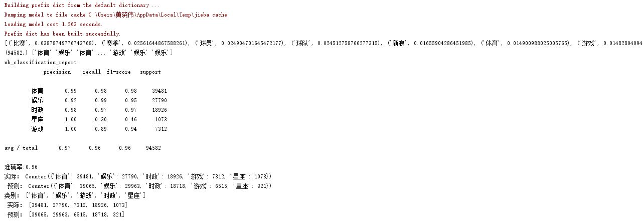
top_value = jieba.analyse.extract_tags(str, topK=10, withWeight=True,allowPOS=())
print(top_value)

#按0.7:0.3比例分为训练集和测试集
from sklearn.model_selection import train_test_split
x_train,x_test,y_train,y_test=train_test_split(all_txt,all_target,test_size=0.3,stratify=all_target)
#将其向量化
from sklearn.feature_extraction.text import TfidfVectorizer
vectorizer=TfidfVectorizer()
X_train=vectorizer.fit_transform(x_train)
X_test=vectorizer.transform(x_test)

#分类结果显示
from sklearn.metrics import confusion_matrix
from sklearn.metrics import classification_report
from sklearn.naive_bayes import  MultinomialNB
mnb=MultinomialNB()#建立模型
clf=mnb.fit(X_train,y_train)#训练模型
#x_test预测结果
y_nb_pred = clf.predict(X_test)
print(y_nb_pred.shape,y_nb_pred)
#主要分类指标的文本报告
print('nb_classification_report:')
cr=classification_report(y_test,y_nb_pred)
print(cr)
#输出精确度
from sklearn.model_selection import cross_val_score
score=cross_val_score(mnb,X_train,y_train,cv=5)
print("准确率:%.2f"%score.mean())

#实际结果与预测结果的对比
import collections
testCount = collections.Counter(y_test)
predCount = collections.Counter(y_nb_pred)
print('实际：',testCount,'\n', '预测：', predCount)

# 建立标签列表，实际结果列表，预测结果列表，
nameList = list(testCount.keys())
testList = list(testCount.values())
predList = list(predCount.values())
x = list(range(len(nameList)))
print("类别：",nameList,'\n',"实际：",testList,'\n',"预测：",predList)

# 对以上数据进行画图显示
import matplotlib.pyplot as plt
from pylab import mpl
mpl.rcParams['font.sans-serif'] = ['youyuan'] # 指定默认字体
plt.figure(figsize=(7,5))
total_width, n = 0.6, 2
width = total_width / n
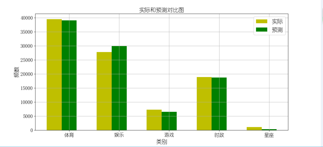
plt.bar(x, testList, width=width,label='实际',fc = 'y')
for i in range(len(x)):
    x[i] = x[i] + width
plt.bar(x, predList,width=width,label='预测',tick_label = nameList,fc='g')
plt.grid()
plt.title('实际和预测对比图',fontsize=17)
plt.xlabel('类别',fontsize=17)
plt.ylabel('频数',fontsize=17)
plt.legend(fontsize =17)
plt.tick_params(labelsize=15)
plt.show()