Coursera--Neural Networks and Deep Learning Week 2

最近在coursera上开坑学习deep learning啦~决定在cnblogs上记载一点心得（其实主要是笔记啦

课程链接： https://www.coursera.org/learn/neural-networks-deep-learning

WEEK 2

主要是用 logistic regression 完成一个识别猫的识别器。

大致思路：

• Build the general architecture of a learning algorithm, including:
  • Initializing parameters
  • Calculating the cost function and its gradient
  • Using an optimization algorithm (gradient descent)
• Gather all three functions above into a main model function, in the right order。

接下来整理一下coursera上notebook的代码和思路：

　　1、学习阶段

　　2、预测

　　

1-packages

import numpy as np
import matplotlib.pyplot as plt
import h5py
import scipy
from PIL import Image
from scipy import ndimage
from lr_utils import load_dataset

%matplotlib inline

　　numpy: fundamental package for scientific computing with Python

　　h5py: to interact with a dataset that is stored on an H5 file

　　matplotlib: plot graphs for analysising datas

2 - Overview of the Problem set

- a training set of m_train images labeled as cat (y=1) or non-cat (y=0)
- a test set of m_test images labeled as cat or non-cat
- each image is of shape (num_px, num_px, 3) where 3 is for the 3 channels (RGB). Thus, each image is square (height = num_px) and (width = num_px).

You will build a simple image-recognition algorithm that can correctly classify pictures as cat or non-cat.

Let's get more familiar with the dataset. Load the data by running the following code.

For convenience, you should now reshape images of shape (num_px, num_px, 3) in a numpy-array of shape (num_px ∗∗ num_px ∗∗ 3, 1). After this, our training (and test) dataset is a numpy-array where each column represents a flattened image. There should be m_train (respectively m_test) columns.

A trick when you want to flatten a matrix X of shape (a,b,c,d) to a matrix X_flatten of shape (b∗∗c∗∗d, a) is to use:

X_flatten = X.reshape(X.shape[0], -1).T      # X.T is the transpose of X

# Reshape the training and test examples

### START CODE HERE ### (≈ 2 lines of code)
train_set_x_flatten = train_set_x_orig.reshape(train_set_x_orig.shape[0],-1).T
test_set_x_flatten = test_set_x_orig.reshape(test_set_x_orig.shape[0],-1).T
### END CODE HERE ###

print ("train_set_x_flatten shape: " + str(train_set_x_flatten.shape))
print ("train_set_y shape: " + str(train_set_y.shape))
print ("test_set_x_flatten shape: " + str(test_set_x_flatten.shape))
print ("test_set_y shape: " + str(test_set_y.shape))
print ("sanity check after reshaping: " + str(train_set_x_flatten[0:5,0]))

To represent color images, the red, green and blue channels (RGB) must be specified for each pixel, and so the pixel value is actually a vector of three numbers ranging from 0 to 255.

One common preprocessing step in machine learning is to center and standardize your dataset, meaning that you substract the mean of the whole numpy array from each example, and then divide each example by the standard deviation of the whole numpy array. But for picture datasets, it is simpler and more convenient and works almost as well to just divide every row of the dataset by 255 (the maximum value of a pixel channel).

Let's standardize our dataset.

train_set_x = train_set_x_flatten/255.
test_set_x = test_set_x_flatten/255.

What you need to remember:

Common steps for pre-processing a new dataset are:

• Figure out the dimensions and shapes of the problem (m_train, m_test, num_px, ...)
• Reshape the datasets such that each example is now a vector of size (num_px * num_px * 3, 1)
• "Standardize" the data

3 - General Architecture of the learning algorithm

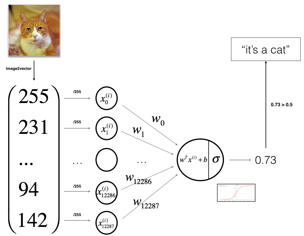
Mathematical expression of the algorithm:

For one example x(i)x(i):

z(i)=wTx(i)+b(1)(1)z(i)=wTx(i)+b

ŷ (i)=a(i)=sigmoid(z(i))(2)(2)y^(i)=a(i)=sigmoid(z(i))

(a(i),y(i))=−y(i)log(a(i))−(1−y(i))log(1−a(i))(3)(3)L(a(i),y(i))=−y(i)log⁡(a(i))−(1−y(i))log⁡(1−a(i))

 

The cost is then computed by summing over all training examples:

J=1m∑i=1m(a(i),y(i))(6)(6)J=1m∑i=1mL(a(i),y(i))

 

Key steps: In this exercise, you will carry out the following steps:

- Initialize the parameters of the model
- Learn the parameters for the model by minimizing the cost  
- Use the learned parameters to make predictions (on the test set)
- Analyse the results and conclude

4 - Building the parts of our algorithm

4.1-helper function (sigmoid)

def sigmoid(z):
    """
    Compute the sigmoid of z

    Arguments:
    z -- A scalar or numpy array of any size.

    Return:
    s -- sigmoid(z)
    """

    ### START CODE HERE ### (≈ 1 line of code)
    s = None
    s=1/(1+np.exp(-1*z))
    ### END CODE HERE ###
    
    return s

4.3-Initializing parameters(using numpy.zeros() to initialize vectors like w)

# GRADED FUNCTION: initialize_with_zeros

def initialize_with_zeros(dim):
    """
    This function creates a vector of zeros of shape (dim, 1) for w and initializes b to 0.
    
    Argument:
    dim -- size of the w vector we want (or number of parameters in this case)
    
    Returns:
    w -- initialized vector of shape (dim, 1)
    b -- initialized scalar (corresponds to the bias)
    """
    
    ### START CODE HERE ### (≈ 1 line of code)
    w = None
    w = np.zeros((dim,1))
    b = None
    b = 0
    ### END CODE HERE ###

    assert(w.shape == (dim, 1))
    assert(isinstance(b, float) or isinstance(b, int))
    
    return w, b

4.3 - Forward and Backward propagation

Now that your parameters are initialized, you can do the "forward" and "backward" propagation steps for learning the parameters.

Implement a function propagate() that computes the cost function and its gradient.

 

# GRADED FUNCTION: propagate

def propagate(w, b, X, Y):
    """
    Implement the cost function and its gradient for the propagation explained above

    Arguments:
    w -- weights, a numpy array of size (num_px * num_px * 3, 1)
    b -- bias, a scalar
    X -- data of size (num_px * num_px * 3, number of examples)
    Y -- true "label" vector (containing 0 if non-cat, 1 if cat) of size (1, number of examples)

    Return:
    cost -- negative log-likelihood cost for logistic regression
    dw -- gradient of the loss with respect to w, thus same shape as w
    db -- gradient of the loss with respect to b, thus same shape as b
    
    Tips:
    - Write your code step by step for the propagation. np.log(), np.dot()
    """
    
    m = X.shape[1]
    
    # FORWARD PROPAGATION (FROM X TO COST)
    ### START CODE HERE ### (≈ 2 lines of code)
    A = sigmoid(np.dot(w.T,X)+b)                                # compute activation
    cost = np.sum(Y*np.log(A)+(1-Y)*np.log(1-A))*(-1)/(m)                                # compute cost
    ### END CODE HERE ###
    
    # BACKWARD PROPAGATION (TO FIND GRAD)
    ### START CODE HERE ### (≈ 2 lines of code)
    dw = np.dot(X,(A-Y).T)/m
   # print("aaa",A)
    db = np.sum(A-Y)/m
    ### END CODE HERE ###

    assert(dw.shape == w.shape)
    assert(db.dtype == float)
    cost = np.squeeze(cost)
    assert(cost.shape == ())
    
    grads = {"dw": dw,
             "db": db}
    
    return grads, cost

4.4 - Optimization

• You have initialized your parameters.
• You are also able to compute a cost function and its gradient.
• Now, you want to update the parameters using gradient descent.

Exercise: Write down the optimization function. The goal is to learn ww and bb by minimizing the cost function JJ. For a parameter θθ, the update rule is θ=θ−α dθθ=θ−α dθ, where αα is the learning rate.

# GRADED FUNCTION: optimize

def optimize(w, b, X, Y, num_iterations, learning_rate, print_cost = False):
    """
    This function optimizes w and b by running a gradient descent algorithm
    
    Arguments:
    w -- weights, a numpy array of size (num_px * num_px * 3, 1)
    b -- bias, a scalar
    X -- data of shape (num_px * num_px * 3, number of examples)
    Y -- true "label" vector (containing 0 if non-cat, 1 if cat), of shape (1, number of examples)
    num_iterations -- number of iterations of the optimization loop
    learning_rate -- learning rate of the gradient descent update rule
    print_cost -- True to print the loss every 100 steps
    
    Returns:
    params -- dictionary containing the weights w and bias b
    grads -- dictionary containing the gradients of the weights and bias with respect to the cost function
    costs -- list of all the costs computed during the optimization, this will be used to plot the learning curve.
    
    Tips:
    You basically need to write down two steps and iterate through them:
        1) Calculate the cost and the gradient for the current parameters. Use propagate().
        2) Update the parameters using gradient descent rule for w and b.
    """
    
    costs = []
    
    for i in range(num_iterations):
        
        
        # Cost and gradient calculation (≈ 1-4 lines of code)
        ### START CODE HERE ### 
        grads,cost = propagate(w, b, X, Y)
        ### END CODE HERE ###
        
        # Retrieve derivatives from grads
        dw = grads["dw"]
        db = grads["db"]
        
        # update rule (≈ 2 lines of code)
        ### START CODE HERE ###
        w = w-dw*learning_rate
        b = b-db*learning_rate
        ### END CODE HERE ###
        
        # Record the costs
        if i % 100 == 0:
            costs.append(cost)
        
        # Print the cost every 100 training iterations
        if print_cost and i % 100 == 0:
            print ("Cost after iteration %i: %f" %(i, cost))
    
    params = {"w": w,
              "b": b}
    
    grads = {"dw": dw,
             "db": db}
    
    return params, grads, costs

Exercise: The previous function will output the learned w and b. We are able to use w and b to predict the labels for a dataset X. Implement the predict() function. There are two steps to computing predictions:

1. Calculate Ŷ =A=σ(wTX+b)Y^=A=σ(wTX+b)

2. Convert the entries of a into 0 (if activation <= 0.5) or 1 (if activation > 0.5), stores the predictions in a vector Y_prediction. If you wish, you can use an if/else statement in a for loop (though there is also a way to vectorize this).

# GRADED FUNCTION: predict

def predict(w, b, X):
    '''
    Predict whether the label is 0 or 1 using learned logistic regression parameters (w, b)
    
    Arguments:
    w -- weights, a numpy array of size (num_px * num_px * 3, 1)
    b -- bias, a scalar
    X -- data of size (num_px * num_px * 3, number of examples)
    
    Returns:
    Y_prediction -- a numpy array (vector) containing all predictions (0/1) for the examples in X
    '''
    
    m = X.shape[1]
    Y_prediction = np.zeros((1,m))
    w = w.reshape(X.shape[0], 1)
    
    # Compute vector "A" predicting the probabilities of a cat being present in the picture
    ### START CODE HERE ### (≈ 1 line of code)
    A = sigmoid(np.dot(w.T,X)+b)
    ### END CODE HERE ###
    
    for i in range(A.shape[1]):
        
        # Convert probabilities A[0,i] to actual predictions p[0,i]
        ### START CODE HERE ### (≈ 4 lines of code)
        if A[0][i]<=0.5:
            Y_prediction[0][i]=0
        else:
            Y_prediction[0][i]=1
        ### END CODE HERE ###
    
    assert(Y_prediction.shape == (1, m))
    
    return Y_prediction

What to remember: You've implemented several functions that:

• Initialize (w,b)
• Optimize the loss iteratively to learn parameters (w,b):Use the learned (w,b) to predict the labels for a given set of examples
  • computing the cost and its gradient
  • updating the parameters using gradient descent

5 - Merge all functions into a model

# GRADED FUNCTION: model

def model(X_train, Y_train, X_test, Y_test, num_iterations = 2000, learning_rate = 0.5, print_cost = False):
    """
    Builds the logistic regression model by calling the function you've implemented previously
    
    Arguments:
    X_train -- training set represented by a numpy array of shape (num_px * num_px * 3, m_train)
    Y_train -- training labels represented by a numpy array (vector) of shape (1, m_train)
    X_test -- test set represented by a numpy array of shape (num_px * num_px * 3, m_test)
    Y_test -- test labels represented by a numpy array (vector) of shape (1, m_test)
    num_iterations -- hyperparameter representing the number of iterations to optimize the parameters
    learning_rate -- hyperparameter representing the learning rate used in the update rule of optimize()
    print_cost -- Set to true to print the cost every 100 iterations
    
    Returns:
    d -- dictionary containing information about the model.
    """
    
    ### START CODE HERE ###
    
    # initialize parameters with zeros (≈ 1 line of code)
    w, b = np.zeros((X_train.shape[0],1)),0
    # Gradient descent (≈ 1 line of code)
    parameters, grads, costs = optimize(w, b, X_train, Y_train, num_iterations, learning_rate, print_cost)
    
    # Retrieve parameters w and b from dictionary "parameters"
    w = parameters["w"]
    b = parameters["b"]
    
    # Predict test/train set examples (≈ 2 lines of code)
    Y_prediction_test = predict(w,b,X_test)
    Y_prediction_train = predict(w,b,X_train)

    ### END CODE HERE ###

    # Print train/test Errors
    print("train accuracy: {} %".format(100 - np.mean(np.abs(Y_prediction_train - Y_train)) * 100))
    print("test accuracy: {} %".format(100 - np.mean(np.abs(Y_prediction_test - Y_test)) * 100))

    
    d = {"costs": costs,
         "Y_prediction_test": Y_prediction_test, 
         "Y_prediction_train" : Y_prediction_train, 
         "w" : w, 
         "b" : b,
         "learning_rate" : learning_rate,
         "num_iterations": num_iterations}
    
    return d

7 - Test with your own image (optional/ungraded exercise)

## START CODE HERE ## (PUT YOUR IMAGE NAME) 
my_image = "my_image.jpg"   # change this to the name of your image file 
## END CODE HERE ##

# We preprocess the image to fit your algorithm.
fname = "images/" + my_image
image = np.array(ndimage.imread(fname, flatten=False))
my_image = scipy.misc.imresize(image, size=(num_px,num_px)).reshape((1, num_px*num_px*3)).T
my_predicted_image = predict(d["w"], d["b"], my_image)

plt.imshow(image)
print("y = " + str(np.squeeze(my_predicted_image)) + ", your algorithm predicts a \"" + classes[int(np.squeeze(my_predicted_image)),].decode("utf-8") +  "\" picture.")

What to remember from this assignment:

• Preprocessing the dataset is important.
• You implemented each function separately: initialize(), propagate(), optimize(). Then you built a model().
• Tuning the learning rate (which is an example of a "hyperparameter") can make a big difference to the algorithm. You will see more examples of this later in this course!