Logistic Regression with a Neural Network mindset
作业简介
本次作业的内容是使用logistic回归来对猫进行分类,你将会了解到创建一个学习算法的基本步骤:
- 参数初始化;
- 计算代价函数与梯度;
- 使用优化函数(在此使用梯度下降);
- 使用一个main函数将上述三个步骤合理的安排在一起。
本次作业使用的数据集下载链接。
工具包
使用下面的代码引入本次作业所需要的所有库:
import numpy as np
import matplotlib.pyplot as plt
import h5py
import scipy
from PIL import Image
from scipy import ndimage
from lr_utils import load_dataset
其中:
- numpy专门用于进行科学计算
- h5py用于跟H5格式的数据库进行交互
- matplotlib是用于绘制图形的库
- PIL,scipy是用来最后使用你自己的图片来验证模型
问题集概述
- 提供数据集("data.h5"),数据集中的内容有:
- 训练集m_train图片,并带有是否是猫的标签
- 测试集m_test图片,并带有是否是猫的标签
- 每个图片的维度都是(num_px,num_px,3),3代表了RGB三个通道,图片都是正方形的,也就是width=height=num_px
我们的目的就是构建一个准确的分类方法,来区分输入的图片究竟是否是猫。
下面我们增进一下对于数据集的了解:
加载数据集
# Loading the data (cat/non-cat)
train_set_x_orig,train_set_y,test_set_x_orig,test_set_y,classes = load_dataset()
之所以在上面的输入后面都加上_orig是因为接下来我们会对输入进行预处理,预处理之后,我们将其命名为train_set_x,test_set_x。
train_set_orig和test_set_orig的每一行数据都代表着一张图片,我们可以采用索引的方式来查看一下这个图片:
# Example of a picture
index = 25
plt.imshow(train_set_orig[index])
print ("y = " + str(train_set_y[:, index]) + ", it's a '" + classes[np.squeeze(train_set_y[:, index])].decode("utf-8") +  "' picture.")
plt.show()
之后程序输出:
y = [1], it's a 'cat' picture.
获取数据集的其它信息
在这里需要注意的是train_set_x_orig的维度是(m_train,num_px,num_px,3):
m_train = train_set_x_orig.shape[0]
m_test = test_set_x_orig.shape[0]
num_px = train_set_x_orig[0].shape[0]

print ("Number of training examples: m_train = " + str(m_train))
print ("Number of testing examples: m_test = " + str(m_test))
print ("Height/Width of each image: num_px = " + str(num_px))
print ("Each image is of size: (" + str(num_px) + ", " + str(num_px) + ", 3)")
print ("train_set_x shape: " + str(train_set_x_orig.shape))
print ("train_set_y shape: " + str(train_set_y.shape))
print ("test_set_x shape: " + str(test_set_x_orig.shape))
print ("test_set_y shape: " + str(test_set_y.shape))
输出:
Number of training examples: m_train = 209
Number of testing examples: m_test = 50
Height/Width of each image: num_px = 64
Each image is of size: (64, 64, 3)
train_set_x shape: (209, 64, 64, 3)
train_set_y shape: (1, 209)
test_set_x shape: (50, 64, 64, 3)
test_set_y shape: (1, 50)
数据预处理
接下来为了方便会对输入数据集的维度进行调整,由原来的(num_px, num_px, 3)调整到 (num_px ∗∗num_px ∗∗ 3, 1),经过这样的调整之后 ,数据集中的每一列都代表了一张图片,所以这里应该有m_train列 。
这里有个技巧,如果你想把矩阵 (a,b,c,d)的维度调整为 (b∗c∗d, a),那么你可以使用下面的方法:
X_flatten = X.reshape(X.shape[0],-1).T # X.T is the transpose of X
按照这个思路,我们将train和test数据集进行调整:
# Reshape the training and test examples
train_set_x_flatten =  train_set_x_orig.reshape(m_train,-1).T
test_set_x_flatten =  test_set_x_orig.reshape(m_test,-1).T

print ("train_set_x_flatten shape: " + str(train_set_x_flatten.shape))
print ("train_set_y shape: " + str(train_set_y.shape))
print ("test_set_x_flatten shape: " + str(test_set_x_flatten.shape))
print ("test_set_y shape: " + str(test_set_y.shape))
print ("sanity check after reshaping: " + str(train_set_x_flatten[0:5,0]))
输出:
train_set_x_flatten shape: (12288, 209)
train_set_y shape: (1, 209)
test_set_x_flatten shape: (12288, 50)
test_set_y shape: (1, 50)
sanity check after reshaping: [17 31 56 22 33]
为了代表彩色图像,需要RGB3个通道,每个通道的像素值都是0-255。
在机器学习中预处理的常见步骤就是数据中心化和标准化,常用的处理方法是对于每个样本都减去均值,然后再除以整个矩阵的标准差。
但是在图像中有一种简单的额归一化方法,效果也不错,就是每个样本都除以255(每个通道像素的最大值)。
归一化图像数据的方法为:
train_set_x = train_set_x_flatten/255.
test_set_x = test_set_x_flatten/255.
学习算法的基本架构
下图展示了logistic回归本质上是简单的神经网络:
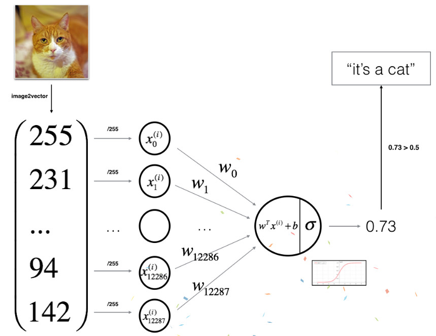
数学表达式为:
对于输入的样本${x^{(i)}}$:

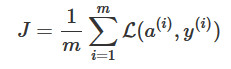
然后,代价函数的计算将对多有的训练样本求和:
创建算法
算法的创建基本流程是:
- 定义模型的架构(比如输入特征的数量)
- 初始化模型参数
- 循环
- 前向传播计算当前的代价函数
- 反向传播计算当前的梯度
- 使用梯度下降的方法更新参数
通常我们会分别实现1-3三个步骤,并且最终放在一个函数model ()中。
辅助函数
sigmoid函数:
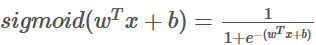
# GRADED FUNCTION: sigmoid
def sigmoid(z):
    s = 1 / (1 + np.exp(-z))
    return s
我们可以测试一下:
print ("sigmoid([0, 2]) = " + str(sigmoid(np.array([0,2]))))
输出:
sigmoid([0, 2]) = [ 0.5 0.88079708]
初始化参数
初始化参数w,b:
# GRADED FUNCTION: initialize_with_zeros
def initialize_with_zeros(dim):
    w = np.zeros((dim, 1))
    b = 0
    assert(w.shape == (dim, 1))
    assert(isinstance(b, float) or isinstance(b, inr))
    return w,b
同样,我们可以测试一下:
dim = 2
w, b = initialize_with_zeros(dim)
print ("w = " + str(w))
print ("b = " + str(b))
输出:
w = [[ 0.]
 [ 0.]]
b = 0
对于图像而言,w的维度应该是 (num_px *num_px *3, 1)
前向传播和反向传播
参数初始化完成之后,就可以采用前向传播和反向传播来学习参数:
对于前向传播:
输入X
可以计算A:

接着计算代价函数J:

然后计算W,b的梯度:
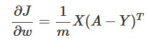
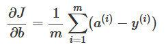
# GRADED FUNCTION: propagate
def propagate(w, b, X, Y):
    m = X.shape[1]
    A = sigmoid(np.dot(w.T,X)+b)
    cost = -1 / m * np.sum(np.multiply(Y, np.log(A)) + np.multiply(1 - Y, np.log(1 - A)))
    dw = 1 / m * np.dot(X,(A-Y).T)
    db = 1 / m * np.sum(A-Y)

    assert(dw.shape == w.shape)
    assert(db.dtype == float)
    cost = np.squeeze(cost)
    assert(cost.shape == ())

    grads = {"dw": dw,
             "db": db}
    return grads, cost
测试:
w, b, X, Y = np.array([[1],[2]]), 2, np.array([[1,2],[3,4]]), np.array([[1,0]])
grads, cost = propagate(w, b, X, Y)
print ("dw = " + str(grads["dw"]))
print ("db = " + str(grads["db"]))
print ("cost = " + str(cost))
输出:
dw = [[ 0.99993216]
 [ 1.99980262]]
db = 0.499935230625
cost = 6.00006477319
参数优化
# GRADED FUNCTION: optimize
def optimize(w, b, X, Y, num_iterations, learning_rate, print_cost = False):
    costs = []
    for i in range(num_iterations):
        grades,cost = propagate(w,b,X,Y)
        dw = grades["dw"]
        db = grades["db"]
        w = w - learning_rate * dw
        b = b - learning_rate * db

        if i % 100 == 0:
            costs.append(cost)
        if print_cost and i % 100 == 0:
            print("Cost after iteration %i: %f" % (i, cost))

    params = {"w": w,
              "b": b}

    grads = {"dw": dw,
             "db": db}

    return params, grads, costs
测试:
params, grads, costs = optimize(w, b, X, Y, num_iterations= 100, learning_rate = 0.009, print_cost = False)
print ("w = " + str(params["w"]))
print ("b = " + str(params["b"]))
print ("dw = " + str(grads["dw"]))
print ("db = " + str(grads["db"]))
输出:
w = [[ 0.1124579 ]
 [ 0.23106775]]
b = 1.55930492484
dw = [[ 0.90158428]
 [ 1.76250842]]
db = 0.430462071679
推测
通过前面的步骤已经可以获得参数w和参数b那么此时就可以进行对任意输入图片进行推测,推测函数为predict(),推测的步骤:
计算:
根据上面式子的结果,可以进行判断例如 0 (if activation <= 0.5) or 1 (if activation > 0.5)。
# GRADED FUNCTION: predict
def predict(w, b, X):
    m = X.shape[1]
    Y_prediction = np.zeros((1,m))
    w = w.reshape(X.shape[0], 1)
    A = sigmoid(np.dot(w.T, X) + b)
    for i in range(A.shape[1]):
        if (A[0, i] > 0.5):
            Y_prediction[0, i] = 1
        else:
            Y_prediction[0, i] = 0

    assert (Y_prediction.shape == (1, m))
    return Y_prediction
测试:
print ("predictions = " + str(predict(w, b, X)))
输出:
predictions = [[ 1. 1.]]
所有的函数合成为一个模型
# GRADED FUNCTION: model
def model(X_train, Y_train, X_test, Y_test, num_iterations = 2000, learning_rate = 0.5, print_cost = False):
    w, b = np.zeros((X_train.shape[0], 1)), 0
    parameters, grads, costs = optimize(w, b, X_train, Y_train, num_iterations, learning_rate, print_cost)
    w = parameters["w"]
    b = parameters["b"]
    Y_prediction_test = predict(w, b, X_test)
    Y_prediction_train = predict(w, b, X_train)
    Y_prediction_test = predict(w, b, X_test)
    Y_prediction_train = predict(w, b, X_train)

    print("train accuracy: {} %".format(100 - np.mean(np.abs(Y_prediction_train - Y_train)) * 100))
    print("test accuracy: {} %".format(100 - np.mean(np.abs(Y_prediction_test - Y_test)) * 100))

    d = {"costs": costs,
         "Y_prediction_test": Y_prediction_test,
         "Y_prediction_train": Y_prediction_train,
         "w": w,
         "b": b,
         "learning_rate": learning_rate,
         "num_iterations": num_iterations}

    return d
测试:
d = model(train_set_x, train_set_y, test_set_x, test_set_y, num_iterations = 2000, learning_rate = 0.005, print_cost = True)
输出:
Cost after iteration 0: 0.693147
Cost after iteration 100: 0.584508
Cost after iteration 200: 0.466949
Cost after iteration 300: 0.376007
Cost after iteration 400: 0.331463
Cost after iteration 500: 0.303273
Cost after iteration 600: 0.279880
Cost after iteration 700: 0.260042
Cost after iteration 800: 0.242941
Cost after iteration 900: 0.228004
Cost after iteration 1000: 0.214820
Cost after iteration 1100: 0.203078
Cost after iteration 1200: 0.192544
Cost after iteration 1300: 0.183033
Cost after iteration 1400: 0.174399
Cost after iteration 1500: 0.166521
Cost after iteration 1600: 0.159305
Cost after iteration 1700: 0.152667
Cost after iteration 1800: 0.146542
Cost after iteration 1900: 0.140872
train accuracy: 99.04306220095694 %
test accuracy: 70.0 %
训练的准确性接近100%,测试的准确性为70%,说明出现了过拟合的情况,后面会介绍方法解决这个问题。
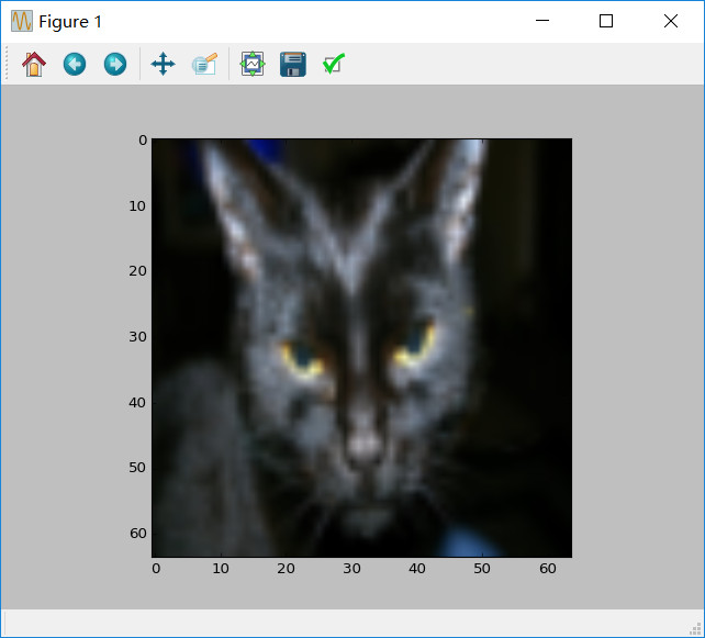
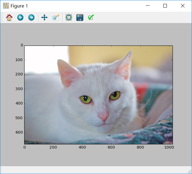
如果想知道测试数据集中具体的图片预测情况:
index = 1
plt.imshow(test_set_x[:,index].reshape((num_px, num_px, 3)))
print ("y = " + str(test_set_y[0,index]) + ", you predicted that it is a \"" + classes[int(d["Y_prediction_test"][0,index])].decode("utf-8") +  "\" picture.")
plt.show()
输出: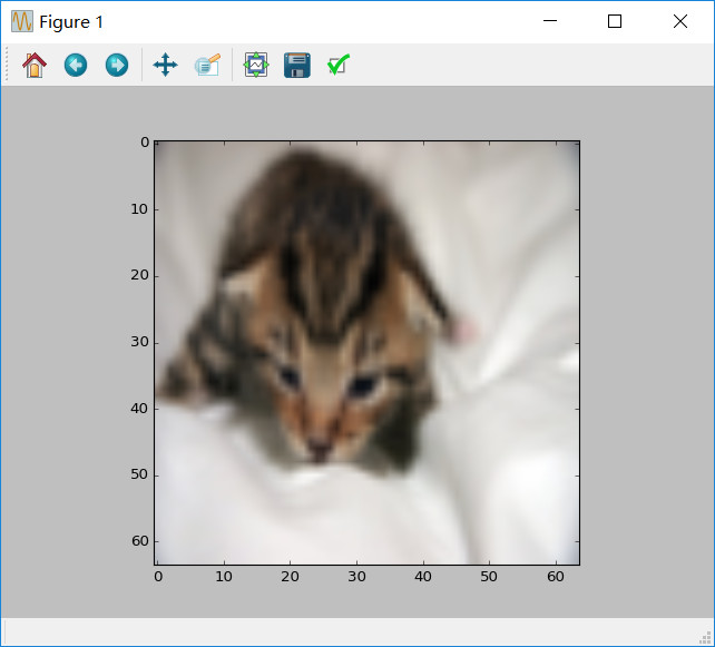
y = 1, you predicted that it is a "cat" picture.
我们还可以打印出梯度和损失函数:
# Plot learning curve (with costs)
costs = np.squeeze(d['costs'])
plt.plot(costs)
plt.ylabel('cost')
plt.xlabel('iterations (per hundreds)')
plt.title("Learning rate =" + str(d["learning_rate"]))
plt.show()
学习率优化
学习率的选取决定了学习的快慢,实际情况我们需要尝试许多种学习率,最终选取效果最好的:
learning_rates = [0.01, 0.001, 0.0001]
models = {}
for i in learning_rates:
    print ("learning rate is: " + str(i))
    models[str(i)] = model(train_set_x, train_set_y, test_set_x, test_set_y, num_iterations = 1500, learning_rate = i, print_cost = False)
    print ('\n' + "-------------------------------------------------------" + '\n')

for i in learning_rates:
    plt.plot(np.squeeze(models[str(i)]["costs"]), label= str(models[str(i)]["learning_rate"]))

plt.ylabel('cost')
plt.xlabel('iterations')

legend = plt.legend(loc='upper center', shadow=True)
frame = legend.get_frame()
frame.set_facecolor('0.90')
plt.show()
输出: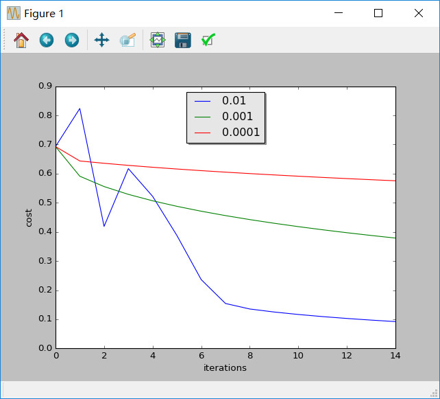
learning rate is: 0.01
train accuracy: 99.52153110047847 %
test accuracy: 68.0 %

-------------------------------------------------------

learning rate is: 0.001
train accuracy: 88.99521531100478 %
test accuracy: 64.0 %

-------------------------------------------------------

learning rate is: 0.0001
train accuracy: 68.42105263157895 %
test accuracy: 36.0 %

-------------------------------------------------------
不同的学习率能够产生不同的代价从而导致不同的预测结果。
学习率如果过大就会导致代价上下震荡(尽管在上面的例子中得到了很好的结果)。
学习率越小并不意味着学习到的模型更好,你需要检查是否出现了过拟合,也就是训练的准确性远远高于测试的准确性。
测试自己的图片
## START CODE HERE ## (PUT YOUR IMAGE NAME)
my_image = "my_image2.jpg"   # change this to the name of your image file
# We preprocess the image to fit your algorithm.
fname = "D:/Anaconda342/assignment2/images/" + my_image
image = np.array(ndimage.imread(fname, flatten=False))
my_image = scipy.misc.imresize(image, size=(num_px,num_px)).reshape((1, num_px*num_px*3)).T
my_predicted_image = predict(d["w"], d["b"], my_image)

plt.imshow(image)
print("y = " + str(np.squeeze(my_predicted_image)) + ", your algorithm predicts a \"" + classes[int(np.squeeze(my_predicted_image)),].decode("utf-8") +  "\" picture.")
注意,上面我使用了自己的图片存储的绝对路径。
输出:
y = 1.0, your algorithm predicts a "cat" picture.