GRU是什么

在LSTM中引入了三个门函数：输入门、遗忘门和输出门。GRU模型中只有两个门：更新门和重置门。

更新门的值越大说明前一时刻的状态信息带入越多。重置门越小，前一状态的信息被写入的越少。

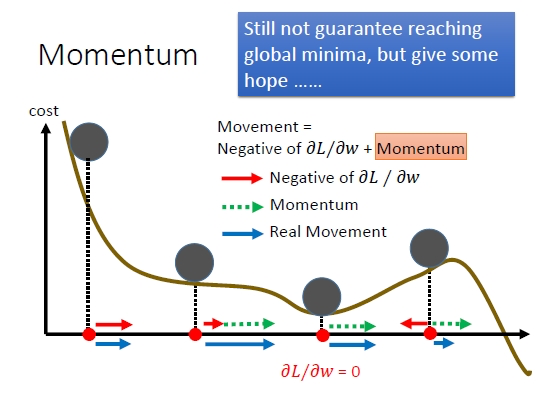
Momentum是什么

梯度下降来求解神经网络的参数，我们在梯度下降时，为了加快收敛速度，通常使用一些优化方法，比如：momentum、RMSprop和Adam等。

SGD每次都会在当前位置上沿着负梯度方向更新，并不考虑之前的方向梯度大小。而动量（moment）通过引入一个新的变量 v，v 去积累之前的梯度（通过指数衰减平均得到）。最直观的理解就是，若当前的梯度方向与累积的历史梯度方向一致，则当前的梯度会被加强，从而这一步下降的幅度更大。若当前的梯度方向与累积的梯度方向不一致，则会减弱当前下降的梯度幅度。红色是梯度方向，绿色是momentum。

下面给出momentum的伪代码：

initialize VdW = 0, vdb = 0 //VdW维度与dW一致，Vdb维度与db一致
on iteration t:
	compute dW,db on current mini-batch（your gradients，beta -- the momentum hyperparameter，一般取值为0.5, 0.9, 0.99。ng推荐取值0.9）

	VdW = beta*VdW + (1-beta)*dW
	Vdb = beta*Vdb + (1-beta)*db
	W = W - learning_rate * VdW
	b = b - learning_rate * Vdb

什么是AdaGrad（Adaptive Gradient）

通常，我们在每一次更新参数时，对于所有的参数使用相同的学习率。而AdaGrad算法的思想是：每一次更新参数时（一次迭代），不同的参数使用不同的学习率。效果是这样就可以使得参数在平缓的地方下降的稍微快些，不至于徘徊不前。但是用的时候要注意，缺点，从训练开始时累积梯度平方会导致学习率过早过量的减少，梯度消失

GW += (dW)^2
W -= learning_rate/(sqrt(GW) + epsilon)*dW
Gb += (db)^2
b -= learning_rate/(sqrt(Gb)+ epsilon)*db

Gt -- python dictionary containing sum of the squares of the gradients up to step t.

#AdaGrad initialization
def initialize_adagrad(parameters):
	L = len(parameters) // 2  # number of layers in the neural networks
	G = {}
	# Initialize velocity
	for l in range(L):
		G["dW" + str(l + 1)] = np.zeros(parameters["W" + str(l + 1)].shape)
		G["db" + str(l + 1)] = np.zeros(parameters["b" + str(l + 1)].shape)
	return G
def update_parameters_with_adagrad(parameters, grads, G, learning_rate, epsilon = 1e-7):
	L = len(parameters) // 2  # number of layers in the neural networks
	# Momentum update for each parameter
	for l in range(L):
		# compute velocities
		G["dW" + str(l + 1)] += grads['dW' + str(l + 1)]**2
		G["db" + str(l + 1)] += grads['db' + str(l + 1)]**2
		# update parameters
		parameters["W" + str(l + 1)] -= learning_rate / (np.sqrt(G["dW" + str(l + 1)]) + epsilon) * grads['dW' + str(l + 1)]
		parameters["b" + str(l + 1)] -= learning_rate / (np.sqrt(G["db" + str(l + 1)]) + epsilon) * grads['db' + str(l + 1)]

	return parameters

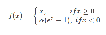
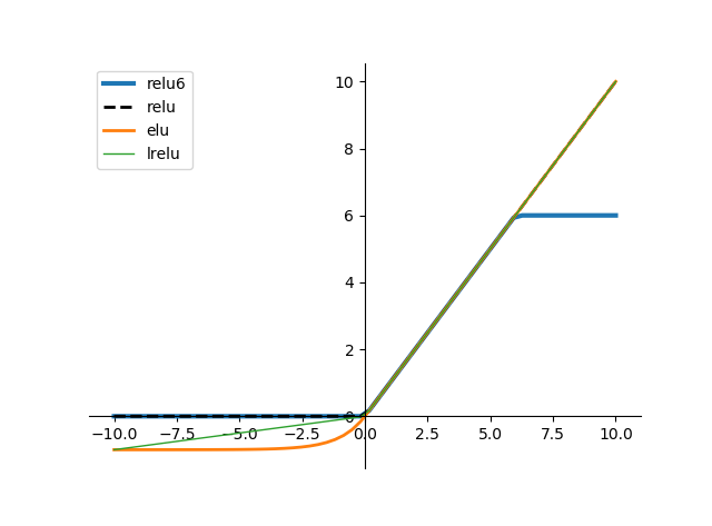
什么是激活函数elu

它结合了sigmoid和ReLU函数（橙色的线），右侧线性部分使得ELU能缓解梯度消失，而左侧软饱和能让对ELU对输入变化或噪声更鲁棒。ELU的输出均值接近于0，所以收敛速度更快。相比于ReLU函数，在输入为负数的情况下，是有一定的输出的，这样可以消除ReLU死掉的问题

input=tf.constant([0,-1,2,-3],dtype=tf.float32)
output=tf.nn.elu(input)

with tf.Session() as sess:
    print('input:')
    print(sess.run(input))
    print('output:')
    print(sess.run(output))
    sess.close()
输出结果：

input:
[ 0. -1. 2. -3.]
output:
[ 0. -0.63212055 2. -0.95021296]

theano语法是什么

theano.function相当于sess.run

import numpy as np
import theano.tensor as T
import theano

#activation function example激活函数的例子
x=T.dmatrix('x')
s=1/(1+T.exp(-x)) #np.exp  这是一个激活函数的式子
logistic=theano.function([x],s)
print(logistic([[0,1],[-2,-3]]))


#multiply output for a function多个输入输出的例子
a,b=T.dmatrices('a','b')
dif=a-b
abs_dif=abs(dif)   #绝对值
square_dif=dif**2  #平方
f=theano.function([a,b],[dif,abs_dif,square_dif])#2个输出
print(f(np.ones((2,2)),np.arange(4).reshape((2,2)) ))



x=theano.shared(np.random.rand(3,),'x')
print x.get_value()
f=theano.function([],updates={x:x+1})#x更新为x+1
f()#执行，这一步不能少，执行了updates才有效
print x.get_value()

为什么要定义共享变量？

定义共享变量的原因在于GPU的使用，如果不定义共享的话，那么当GPU调用这些变量时，遇到一次就要调用一次，这样就会花费大量时间在数据存取上，导致使用GPU代码运行很慢，甚至比仅用CPU还慢。shared变量可以通过.set_value()和.get_value()设置和读取状态值

共享变量的类型必须为floatX
因为GPU要求在floatX上操作，所以所有的共享变量都要声明为floatX类型

shared_x = theano.shared(numpy.asarray(data_x, dtype=theano.config.floatX)) 
self.A = theano.shared(name = "A", value = E.astype(theano.config.floatX))

创建tensor variables
在创建变量时可以给变量命名，命名能够加快debugging的过程，所有的构造器中都有name参数供命名

broadcastable是什么

这个东西是一个布尔有元素组成的元组，比如[False,True,False]。

For dimensions in which broadcasting is False, the length of this dimension can be 1 or more.
For dimension in which broadcasting is True, the length of this dimension must be 1

shared变量默认的是broadcastable=False,所以要想使用broadcasrable pattern，需要特别指定，如
theano.shared(...,broadcastable=(True,False))

softmax_neg是在算什么

def softmax_neg(self, X):
        hm = 1.0 - T.eye(*X.shape)
        X = X * hm
        e_x = T.exp(X - X.max(axis=1).dimshuffle(0, 'x')) * hm
        return e_x / e_x.sum(axis=1).dimshuffle(0, 'x')

[0,1],
[-2,-3]


1.0 - T.eye(*X.shape)得到：

[[0. 1.]
 [1. 0.]]


X = X * hm 得到（对应每个元素相乘）（把X的正对角元素拿出来，其余是0）

[[ 0.  1.]
 [-2. -0.]]

X.max(axis=1).dimshuffle(0, 'x') 得到（axis=1是沿着列方向最大，就是每一行的最大）
[[ 1.]
 [-0.]]

这里是每一元素减去每一行的最大值），

[[-1.  0.]
 [-2.  0.]]


 T.exp(X - X.max(axis=1).dimshuffle(0, 'x'))。函数e^x
[[0.36787944 1.        ]
 [0.13533528 1.        ]]

T.exp(X - X.max(axis=1).dimshuffle(0, 'x')) * hm。再把正对焦元素拿出来
[[0.         1.        ]
 [0.13533528 0.        ]]


e_x / e_x.sum(axis=1).dimshuffle(0, 'x'). 分母是每行加起来
[[1.        ]
 [0.13533528]]

整体是
[[0. 1.]
 [1. 0.]]

tf怎么看运算结果？

initialize_all_variables之后sess.run给print out
使用tf.Variable时，如果检测到命名冲突，系统会自己处理。使用tf.get_variable()时，系统不会处理冲突，而会报错

value = [1, 1, 1, 1, -8, 1, 1, 1,1]
init = tf.constant_initializer(value)
W = tf.get_variable('W', shape=[3, 3], initializer=init)
init_op = tf.initialize_all_variables()

with tf.Session() as sess:
    sess.run(init_op)
    print('output:')
    print(sess.run(W))

    sess.close()


output:
[[ 1.  1.  1.]
 [ 1. -8.  1.]
 [ 1.  1.  1.]]

posted @ 2019-09-19 16:01 SENTIMENT_SONNE 阅读(623) 评论(0) 编辑收藏举报

会员力量，点亮园子希望

刷新页面返回顶部

SENTIMENT_SONNE

【深度学习】【论文学习】【推荐系统】 Session-Based Recommendation