


Abstract : The goals of this lecture is to use the level set framework in order to do curve evolution. The mean curvature motion is the basic tool, and it can be extended into edge-based (geodesic active contours) and region-based (Chan-Vese) snakes.
Setting up Matlab.
- First download the Matlab toolbox toolbox_fast_marching.zip. Unzip it into your working directory. You should have a directory toolbox_fast_marching/ in your path.
- The first thing to do is to install this toolbox in your path.
path(path, 'toolbox_fast_marching/');
path(path, 'toolbox_fast_marching/data/');
path(path, 'toolbox_fast_marching/toolbox/'); - Recompile the mex file for your machine (this can produce some warning). If it does not work, either use the already compiled mex file (they should be available in toolbox_fast_marching/ for MacOs and Unix) or try to set up matlab with a C compiler (e.g. gcc) using 'mex -setup'.
cd toolbox_fast_marching
compile_mex;
cd ..
Managing level set function.
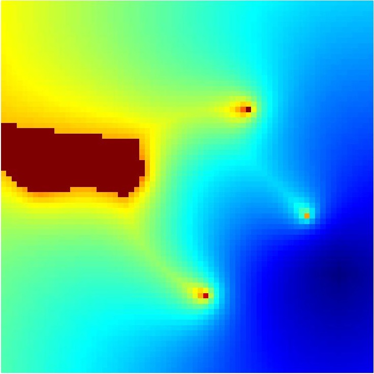
- In order to perform curve evolution, we will deal with a distance function stored in a 2D image D. The curve will be embedded in the level set D=0. This curve will be evolved by modifying the image D. A curve evolution ODE can be replaced by an PDE on D. This allows to deal with topological changes when a curve split or two curves merge.
n = 200; % size of the image
% load a distance function
D0 = compute_levelset_shape('circlerect2', n);
% type 'help compute_levelset_shape' to see other
% basic curve you can load.
% display the curve
clf; hold on;
imagesc(D); axis image; axis off; axis([1 n 1 n]);
[c,h] = contour(D,[0 0], 'r');
set(h, 'LineWidth', 2);
hold off;
colormap gray(256);
% do the union of two curves
options.center = [0.15 0.15]*n;
options.radius = 0.1*n;
D1 = compute_levelset_shape('circle', n,options);
imagesc(min(D0,D1)<0); - During the curve evolution, the image D might become far from being a distance function. In order to stabilize the algorithm, one needs to re-compute this distance function.
% here we simulate a modification of the distance function
[Y,X] = meshgrid(1:n,1:n);
D = (D0.^3) .* (X+n/3);
D1 = perform_redistancing(D);
% display both the original and the new,
% redistanced, curve (should be very close)
...
Mean Curvature Motion.
- In order to compute differential quantities (tangent, normal, curvature, etc) on the curve, you can compute derivatives of the image D.
% the gradient
g0 = divgrad(D);
% display the gradient (as arrow field with 'quiver', ...)
...
% the normalized gradient
d = max(eps, sqrt(sum(g0.^2,3)) );
g = g0 ./ repmat( d, [1 1 2] );
% display
...
% the curvature
K = d .* divgrad( g );
% display
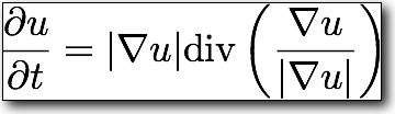
... - The mean curvature motion of the level sets of some image u is driven be the following equation.
Implement this evolution explicitly in time using finite differences.
Tmax = 1000; % maximum time of evolution
dt = 0.4; % time step (should be small)
niter = round(Tmax/dt); % number of iterations
D = D0; % initialization
for i=1:niter
% compute the right hand size of the PDE
...
% update the distance field
D = ...;
% redistance the function from time to time
if mod(i,30)==0
D = perform_redistancing(D);
end
% display from time to time
if mod(i,30)==1
% display here
...
end
end
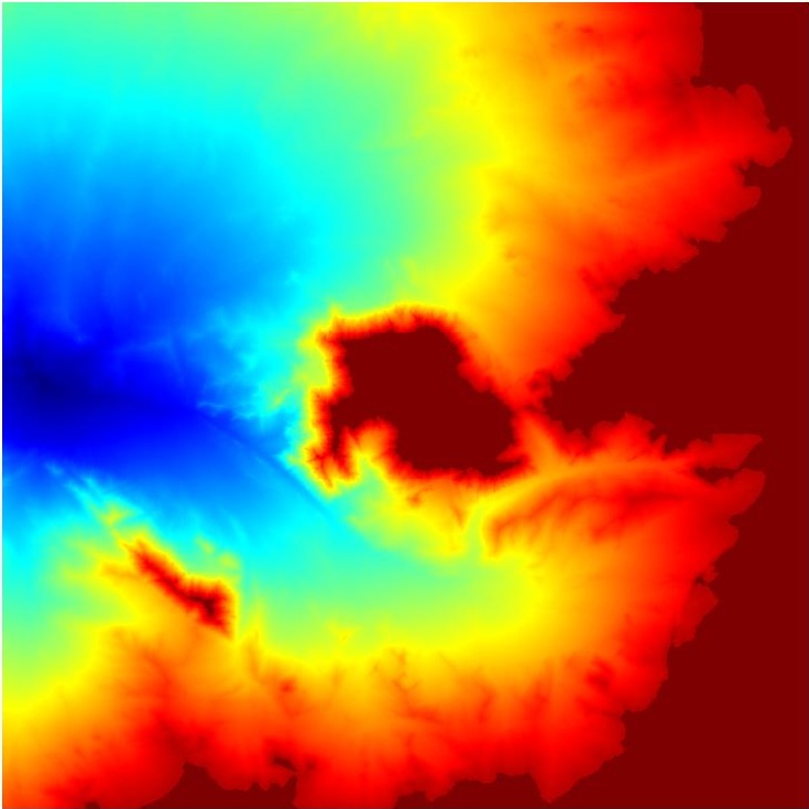

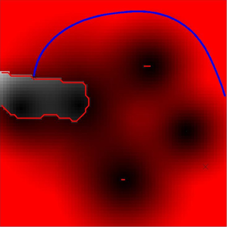
Curve evolution under the mean curvature motion (the background is the distance function D).
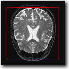
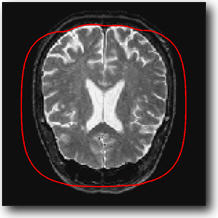
Edge-based Segmentation with Geodesic Active Contour (snakes + level set).
- Given a background image M to segment, one needs to compute an edge-stopping function E. It should be small in area of high gradient, and high in area of large gradient.
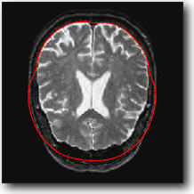
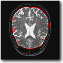
% load an image
name = 'brain';
M = rescale( sum( load_image(name, n), 3) );
% display it
...
% compute a smoothed gradient
sigma = 4; % blurring size
G = divgrad( perform_blurring(M,sigma) );
% compute the norm of the gradient
d = ...
% compute the edge-stopping function
E = 1./max(d, 1e-3);
% rescale it so that it is in realistic ranges
E = rescale(E,0.3,1); - The geodesic active contour evolution is a mean curvature motion modulated by the edge-stopping function:

Implement this evolution explicitly in time using finite differences [warning: the g in the formula is the edge stopping function E].% initialize the level set
D0 = compute_levelset_shape('square', n);
% precompute the gradient of E [which is g in the formula]
...
% do the iterations
...
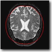
Region-based Segmentation with Chan-Vese (Mumord-Shah + level sets).
- The geodesic active contour uses an edge-based energy. It has lots of local minima and is very sensitive to initialization. In order to circumvent these drawbacks, one can use a region based energy like the Mumford-Shah functional. Re-casted into the level set framework, it reads:
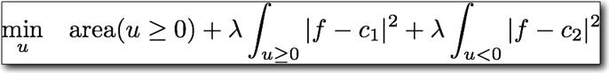
The corresponding gradient descent is the Chan-Vese active contour method:
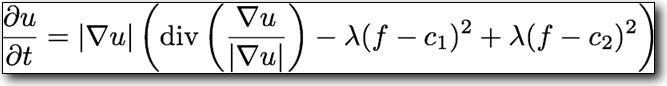
Implement this evolution explicitly in time using finite differences, when c1 and c2 are known in advanced.
% initialize with a complex distance function
D0 = compute_levelset_shape('small-disks', n);
% set parameters
lambda = 0.8;
c1 = ...; % black
c2 = ...; % gray
...

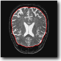
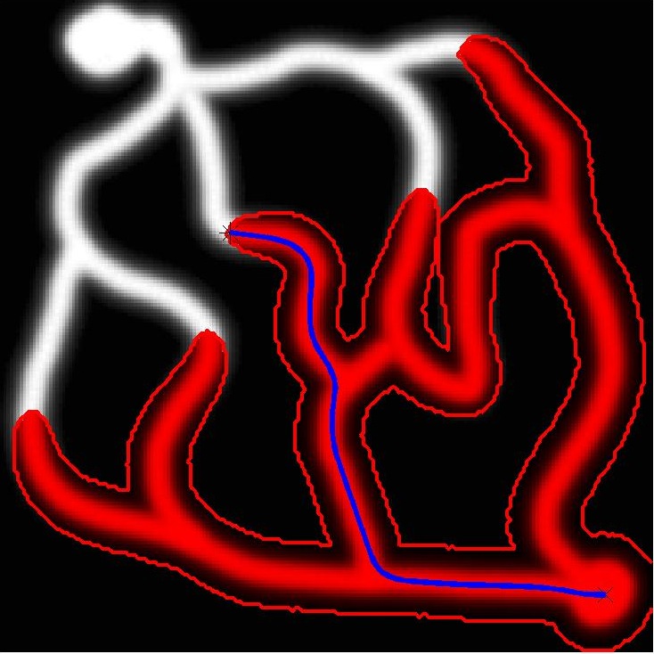
| Segmentation with Chan-Vese active contour without edges. |
Copyright © 2006 Gabriel Peyré
