

机器学习基础(一)线性回归
线性回归模型是最简单的监督式学习模型:

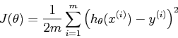
所谓的监督式学习模型就是需要通过已有的数据训练出一个最优的模型,能够表示这些已有的模型并能够预测新的数据。怎么判断模型是不是最优的呢?这就需要引入代价函数(Cost Function):
怎么得到最优的模型呢?这就需要求解代价函数的最小值,也就需要引入梯度下降法。梯度下降法就是通过迭代,每一次都比之前已次更加接近代价函数的最小值,最后在误差允许的范围内终止迭代。

我们求出了参数,带入
便得到了最简单的线性回归模型
参考练习:http://openclassroom.stanford.edu/MainFolder/DocumentPage.php?course=MachineLearning&doc=exercises/ex2/ex2.html
 1 function Linear_Regression()
 2 clear all; close all;clc
 3 x=load('ex2x.dat')
 4 y=load('ex2y.dat')
 5
 6 m=length(y);
 7
 8 %plot the training data
 9 figure;
10 plot(x,y,'o');
11 ylabel('Height in meters');
12 xlabel('Age in years')
13
14 %gradient descent
15 x=[ones(m,1) x];
16 theta = zeros(size(x(1,:)))';
17 MAX_ITER = 1500;
18 alpha=0.07;
19
20 for iter=1:MAX_ITER
21     grad = (1/m).*x'*((x*theta)-y);
22     theta = theta - alpha .*grad;
23 end
24 theta
25
26 hold on;
27 plot(x(:,2),x*theta,'-')
28 legend('Training data','Linear regression')
29 hold off
30
31 predict1=[1,3.5]*theta
32 predict2=[1,7]*theta
33
34 theta0_vals=linspace(-3,3,100);
35 theta1_vals=linspace(-1,1,100);
36
37 J_vals =zeros(length(theta0_vals),length(theta1_vals));
38
39 for i=1:length(theta0_vals)
40     for j=1:length(theta1_vals)
41         t=[theta0_vals(i);theta1_vals(j)];
42         J_vals(i,j) = (0.5/m).*(x*t-y)'*(x*t-y);
43     end
44 end
45 J_vals=  J_vals';
46 figure;
47 surf(theta0_vals,theta1_vals,J_vals)
48 xlabel('\theta_0'); ylabel('\theta_1');
49
50 figure
51 contour(theta0_vals,theta1_vals,J_vals,logspace(-2,2,15))
52 xlabel('\theta_0'); ylabel('\theta_1');
53 end
Cantor图
参考资料http://openclassroom.stanford.edu/MainFolder/CoursePage.php?course=MachineLearning
