机器学习一（决策树和随机森林）

 

前言

本文试图提纲挈领的对决策树和随机森林的原理及应用做以分析

决策树

算法伪代码

def 创建决策树:
    
    if (数据集中所有样本分类一致): #或者其他终止条件
        创建携带类标签的叶子节点
    else:
        寻找划分数据集的最好特征
        根据最好特征划分数据集
        for 每个划分的数据集:
            创建决策子树(递归)

注意算法要采用递归的方法

依据选取划分数据集特征的方法，有三种常用方法：

ID3:信息增益

 

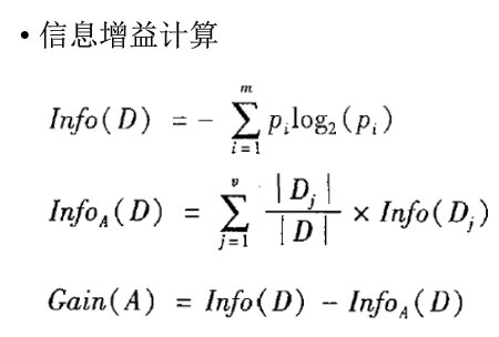
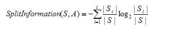
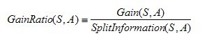
C4.5:信息增益率

 

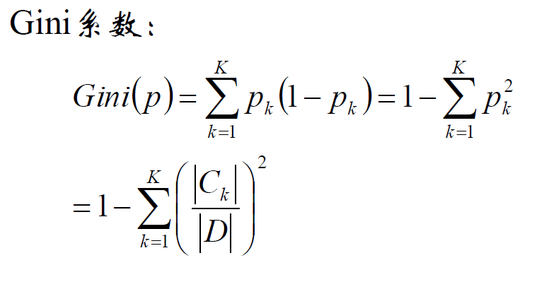
CART:基尼系数

对于连续特征：

比如m个样本的连续特征A有m个，从小到大排列为a1,a2,...,am,则CART算法取相邻两样本值的中位数，一共取得m-1个划分点，其中第i个划分点Ti表示Ti表示为：Ti=(ai+ai+1)/2。对于这m-1个点，分别计算以该点作为二元分类点时的基尼系数。选择基尼系数最小的点作为该连续特征的二元离散分类点，这样我们就做到了连续特征的离散化。要注意的是，与离散属性不同的是，如果当前节点为连续属性，则该属性后面还可以参与子节点的产生选择过程。

过拟合问题-——剪枝

 过多的枝叶会导致算法的过拟合，所以常使用减枝的方法防止过拟合：常用的剪枝方法有前置法和后置法，前置法指的是在要构建决策树时，依据终止条件确定是否提前终止；后置法指构建好决策树后，再依据条件确定是否用单一节点代替子树。

回归问题

一般采用均方误差作为评价特征的标准

随机森林

bootstrap方法：从样本集进行有放回的重采样。

随机森林步骤：

1.  样本的随机：从样本集中用Bootstrap随机选取n个样本

2.  特征的随机：从所有属性中随机选取K个属性，选择最佳分割属性作为节点建立CART决策树

3.  重复以上两步m次，即建立了m棵CART决策树

4.  这m个CART形成随机森林，通过投票表决结果，决定数据属于哪一类（投票机制有一票否决制、少数服从多数、加权多数）

参考：https://www.cnblogs.com/fionacai/p/5894142.html

sklearn.tree.DecisionTreeClassifier

class sklearn.tree.DecisionTreeClassifier(criterion=’gini’, splitter=’best’, max_depth=None, min_samples_split=2, min_samples_leaf=1, min_weight_fraction_leaf=0.0, max_features=None, random_state=None, max_leaf_nodes=None, min_impurity_decrease=0.0, min_impurity_split=None, class_weight=None, presort=False)

 Parameters: criterion='gini' or 'entropy'

                    max_depth 设置树的最大深度 默认为‘None’

                    min_sample_split 分割的最小样本数 默认为2

                    详细内容的中文说明可以参考  https://www.cnblogs.com/pinard/p/6056319.html

 

sklearn.tree.DecisionTreeRegressor

 Parameters: criterion='mse'  还可以使用‘friedman_mse’或者'mae'

                     max_depth 设置树的最大深度 默认为‘None’

 

sklearn.ensemble.RandomForestClassifier

Parameters: n_estimator=10 生成决策树的个数

                   criterion='gini' or 'entropy'

 

应用举例

使用随机森林进行回归的例子

import numpy as np
import matplotlib.pyplot as plt
from sklearn.tree import DecisionTreeRegressor


N=100
x = np.random.rand(N) * 6 - 3 
x.sort()
y=0.1*x**3+np.exp(-x*x/2)+ np.random.randn(N) * 0.2  #3次函数+高斯函数+噪声
x = x.reshape(-1, 1)
x_bar=np.linspace(-3,3,50).reshape(-1,1)
y_bar=0.1*x_bar**3+np.exp(-x_bar*x_bar/2)
plt.plot(x,y,'r.')
plt.plot(x_bar,y_bar)
plt.show()

plt.plot(x,y,'r.')
x_test=np.linspace(-3,3,50).reshape(-1,1)
dt = DecisionTreeRegressor(criterion='mse')
depth=[3,6,18]
color='rgy'
for d,c in zip(depth,color):
    dt.set_params(max_depth=d)
    dt.fit(x, y)
    y_test = dt.predict(x_test)
    plt.plot(x_test,y_test,'-',color=c, linewidth=2, label='Depth=%d' % d)

plt.legend(loc='upper left')
plt.xlabel(u'X')
plt.ylabel(u'Y')
plt.grid(b=True)
plt.show()

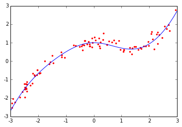　　 图1

 

 

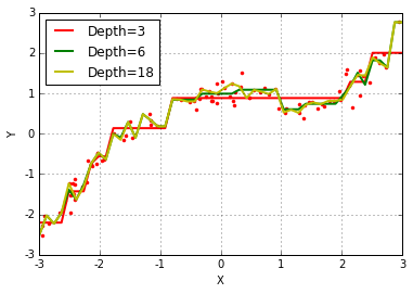
  图2

对比图1中的真实曲线和图2中三条拟合折线可以发现，图二中的折现较好的拟合了原始曲线，如果单纯使用一次特征的线性回归肯定是达不到这样的效果的，其次，我们可以看到当树最大深度为3时，折线段较少，细小的弯曲无法体现，而当深度达到18时，折线波折又过多，有过拟合的嫌疑，当深度为6时，相对较好，因此，我们推断树的深度在拟合过程中起到了重要作用。

 

数据集 Adult

字段名	含义	类型
age	年龄	Double
workclass	工作类型	string
fnlwgt	序号	string
education	教育程度*	string
education_num	受教育时间	double
maritial_status	婚姻状况*	string
occupation	职业*	string
relationship	关系*	string
race	种族*	string
sex	性别*	string
capital_gain	资本收益	string
capital_loss	资本损失	string
hours_per_week	每周工作小时数	double
native_country	国籍	string
income	收入	string

表1

基于上面特征，预测收入是否大于50K，我们用决策树和随机森林来解决上述问题。

import pandas as pd
from sklearn.ensemble import RandomForestClassifier
from sklearn.metrics import accuracy_score
from sklearn.model_selection import train_test_split
from sklearn.tree import DecisionTreeClassifier
from sklearn.linear_model import LogisticRegression
from sklearn.preprocessing import LabelEncoder

column_names = 'age', 'workclass', 'fnlwgt', 'education', 'education-num', 'marital-status', 'occupation', \
                   'relationship', 'race', 'sex', 'capital-gain', 'capital-loss', 'hours-per-week',\
                   'native-country', 'income'  #不加括号为元组
data = pd.read_csv('adult.data', header=None, names=column_names)                  
data.isnull().any().any() #是否存在null
for name in column_names:
    data[name]=LabelEncoder().fit_transform(data[name])   #自动转换非数字列为数字
x = data[data.columns[:-1]]
y = data[data.columns[-1]]    
x_train, x_valid, y_train, y_valid = train_test_split(x, y, test_size=0.3, random_state=0)
DT = DecisionTreeClassifier(criterion='gini',max_depth=10,min_samples_split=5)
RF = RandomForestClassifier(criterion='gini', max_depth=10, min_samples_split=5,n_estimators=20)
LR= LogisticRegression()
models=[DT,RF,LR]
for model in models:
    model.fit(x_train,y_train)
    y_pre=model.predict(x_valid)
    print('验证集准确率：', accuracy_score(y_pre, y_valid))

运行结果为：

验证集准确率： 0.852287849319
验证集准确率： 0.858429726686
验证集准确率： 0.805507216706

对比结果，在随机森林与决策树选取相似的参数时，随机森林的结果略好于决策树，logistic回归结果最差，但注意这里logistic回归没有调参。

附:Adult数据集 https://pan.baidu.com/s/1vTMN9Yp6VPndezUR1UtYtw

 

致谢：本文基于小象学院邹博老师机器学习课程，部分代码参考该课程，特此感谢。